Validation against published newsvendor optima • alloscore2

library(alloscore2)
library(dplyr)
library(purrr)

Acknowledgment

This vignette adapts content from the original alloscore package written by Aaron Gerding, specifically from a vignette that shows how to reproduce results from Zhang, Xu and Hua (2009).

This vignette was drafted by Claude Code (Opus 5) and reviewed for accuracy by Nick Reich.

Why the newsvendor problem

The optimization inside [allocate()] is not specific to forecast evaluation. It solves a budget-constrained separable convex program, and one classical instance of that is the multiproduct newsboy problem with a budget constraint: choose stock levels for several products, under uncertain demand, subject to a limit on total purchasing cost.

That is useful here because the problem has a published literature with reported optima. Zhang, Xu and Hua (2009) give two worked examples, and this package ships their data in zxh_tab2 and zxh_tab3. Reproducing their Opt column checks allocate() against an external source rather than against the package’s own history.

zxh_tab2
#>    Product  v h  c  mu sigma  q_zxh    GIM    Opt
#> 1        1  7 1  4 102  51.0  85.75   0.00   0.00
#> 2        2 12 2  8  73  18.3  62.64   0.00   0.00
#> 3        3 30 4 19 123  30.8 108.90   0.00   0.00
#> 4        4 30 4 17  95  23.8  87.88   0.00   0.00
#> 5        5 40 2 23  62  15.5  58.26   0.00   0.00
#> 6        6 45 5 15 129  43.0 139.89 106.86 106.85
#> 7        7 16 1 10  69  34.5  55.98   0.00   0.00
#> 8        8 21 2 10  83  41.5  80.74  14.02  14.01
#> 9        9 42 3 40 120  30.0  68.96   0.00   0.00
#> 10      10 34 5 20  89  22.3  80.95   0.00   0.00
#> 11      11 20 3 10 115  38.3 108.71  15.58  15.65
#> 12      12 15 5  7  91  30.3  83.32  42.20  42.25
#> 13      13 10 3  4  52  17.3  50.33  34.56  34.60
#> 14      14 20 3 12  76  38.0  61.14   0.00   0.00
#> 15      15 47 2 33  66  16.5  56.66   0.00   0.00
#> 16      16 35 4 21 147  36.8 133.71   0.00   0.00
#> 17      17 22 1 11 104  34.7 102.11  15.23  15.13

From newsvendor costs to gpl parameters

The newsvendor parameterization uses three costs per product: c per unit purchased, v per unit of unmet demand, and h per unit left over. The gpl loss instead uses a scale kappa and a level alpha. stdize_news_params() converts between them, giving

$\kappa = h + v, \qquad \alpha = \frac{v - c}{h + v}.$

The alpha that falls out is the newsvendor’s familiar critical ratio, and the unconstrained optimum is the alpha-quantile of demand.

zxh_norm <- zxh_tab2 |>
  mutate(stdize_news_params(ax = c, a_minus = v, a_plus = h), .after = c) |>
  as_tibble()
zxh_norm |> select(Product, c, v, h, kappa, alpha, q_zxh)
#> # A tibble: 17 × 7
#>    Product     c     v     h kappa  alpha q_zxh
#>    <chr>   <int> <int> <int> <dbl>  <dbl> <dbl>
#>  1 1           4     7     1     8 0.375   85.8
#>  2 2           8    12     2    14 0.286   62.6
#>  3 3          19    30     4    34 0.324  109. 
#>  4 4          17    30     4    34 0.382   87.9
#>  5 5          23    40     2    42 0.405   58.3
#>  6 6          15    45     5    50 0.6    140. 
#>  7 7          10    16     1    17 0.353   56.0
#>  8 8          10    21     2    23 0.478   80.7
#>  9 9          40    42     3    45 0.0444  69.0
#> 10 10         20    34     5    39 0.359   81.0
#> 11 11         10    20     3    23 0.435  109. 
#> 12 12          7    15     5    20 0.4     83.3
#> 13 13          4    10     3    13 0.462   50.3
#> 14 14         12    20     3    23 0.348   61.1
#> 15 15         33    47     2    49 0.286   56.7
#> 16 16         21    35     4    39 0.359  134. 
#> 17 17         11    22     1    23 0.478  102.

Building the demand distributions

Demand is Normal here, so add_pdqr_funs() builds the cdf and quantile function from mean and sd columns. Evaluating each quantile function at its own alpha should recover the critical quantile that Zhang, Xu and Hua print in q_zxh.

zxh_norm_forecasts <- zxh_norm |>
  rename(mean = mu, sd = sigma) |>
  add_pdqr_funs(dist = "norm", types = c("p", "q")) |>
  mutate(q_ours = map2_dbl(Q, alpha, function(Q, alpha) Q(alpha)))

zxh_norm_forecasts |>
  select(Product, alpha, q_zxh, q_ours) |>
  mutate(difference = q_ours - q_zxh)
#> # A tibble: 17 × 5
#>    Product  alpha q_zxh q_ours difference
#>    <chr>    <dbl> <dbl>  <dbl>      <dbl>
#>  1 1       0.375   85.8   85.7 -0.000608 
#>  2 2       0.286   62.6   62.6  0.00314  
#>  3 3       0.324  109.   109.  -0.00184  
#>  4 4       0.382   87.9   87.9 -0.00350  
#>  5 5       0.405   58.3   58.3  0.00387  
#>  6 6       0.6    140.   140.   0.00393  
#>  7 7       0.353   56.0   56.0 -0.0000221
#>  8 8       0.478   80.7   80.7 -0.00253  
#>  9 9       0.0444  69.0   69.0  0.00135  
#> 10 10      0.359   81.0   80.9 -0.00480  
#> 11 11      0.435  109.   109.   0.000727 
#> 12 12      0.4     83.3   83.3  0.00358  
#> 13 13      0.462   50.3   50.3 -0.000464 
#> 14 14      0.348   61.1   61.1 -0.00546  
#> 15 15      0.286   56.7   56.7  0.00184  
#> 16 16      0.359  134.   134.  -0.00222  
#> 17 17      0.478  102.   102.  -0.00181

Allocating under the budget

Zhang, Xu and Hua use a budget of 2500, with the unit cost c as the weight in the constraint. Passing w = "c" tells allocate() to take the weights from that column, and target_names = "Product" names the targets from another.

allo_norm <- allocate(
  zxh_norm_forecasts,
  w = "c",
  K = 2500,
  target_names = "Product"
)

comparison <- zxh_norm_forecasts |>
  select(Product, c, GIM, Opt) |>
  left_join(allo_norm$xdf[[1]], by = "Product") |>
  select(Product, c, GIM, Opt, ours = x) |>
  mutate(difference = ours - Opt)
comparison
#> # A tibble: 17 × 6
#>    Product     c   GIM   Opt  ours difference
#>    <chr>   <int> <dbl> <dbl> <dbl>      <dbl>
#>  1 1           4   0     0     0      0      
#>  2 2           8   0     0     0      0      
#>  3 3          19   0     0     0      0      
#>  4 4          17   0     0     0      0      
#>  5 5          23   0     0     0      0      
#>  6 6          15 107.  107.  107.     0.00635
#>  7 7          10   0     0     0      0      
#>  8 8          10  14.0  14.0  14.0    0.0113 
#>  9 9          40   0     0     0      0      
#> 10 10         20   0     0     0      0      
#> 11 11         10  15.6  15.6  15.7    0.0573 
#> 12 12          7  42.2  42.2  42.3    0.00483
#> 13 13          4  34.6  34.6  34.6   -0.00307
#> 14 14         12   0     0     0      0      
#> 15 15         33   0     0     0      0      
#> 16 16         21   0     0     0      0      
#> 17 17         11  15.2  15.1  15.2    0.0547

Two things to note. Only 6 of the 17 products are stocked at all, and they are exactly the 6 that Zhang, Xu and Hua stock — the budget binds hard enough that most products are shut out entirely, which is a useful test of the boundary handling. And the agreement is to within about a twentieth of a unit:

c(
  max_abs_difference = max(abs(comparison$difference)),
  budget_spent = sum(comparison$c * comparison$ours),
  budget_available = 2500,
  n_stocked_ours = sum(comparison$ours > 1e-8),
  n_stocked_zxh = sum(comparison$Opt > 0)
)
#> max_abs_difference       budget_spent   budget_available     n_stocked_ours 
#>       5.733212e-02       2.501335e+03       2.500000e+03       6.000000e+00 
#>      n_stocked_zxh 
#>       6.000000e+00

The budget is spent to slightly over 2500. That is the eps_K tolerance, 1% by default: the bisection stops once the constraint is satisfied to within that relative tolerance rather than exactly.

Comparing objective values

The comparison that really matters is not the allocation vector but the value of the objective, since the problem can have near-flat optima. exp_gpl_loss_fun() builds the expected loss for one product, including the purchasing cost as an offset.

objective <- function(x) {
  sum(pmap_dbl(
    list(
      zxh_norm_forecasts$F,
      zxh_norm_forecasts$kappa,
      zxh_norm_forecasts$alpha,
      zxh_norm_forecasts$mean,
      zxh_norm_forecasts$c,
      x
    ),
    function(F, kappa, alpha, mean, c, x) {
      exp_gpl_loss_fun(F = F, kappa = kappa, alpha = alpha, offset = c * mean)(x)
    }
  ))
}

c(
  objective_at_zxh_opt = objective(comparison$Opt),
  objective_at_ours = objective(comparison$ours),
  objective_at_gim = objective(comparison$GIM)
)
#> objective_at_zxh_opt    objective_at_ours     objective_at_gim 
#>             39825.18             39823.79             39825.04

Our objective value is marginally lower than at the published optimum, which is what the slight overspend buys. Both are below the earlier Abdel-Malek and Montanari solution in the GIM column.

The search

plot_iterations() shows the bisection on the shadow price of the budget. With the default tolerances it takes 15 steps, the last few of which barely move the allocation.

plot_iterations(allo_norm, num_targets_to_color = 6)
#> Warning: Removed 1 row containing missing values or values outside the scale range
#> (`geom_ribbon()`).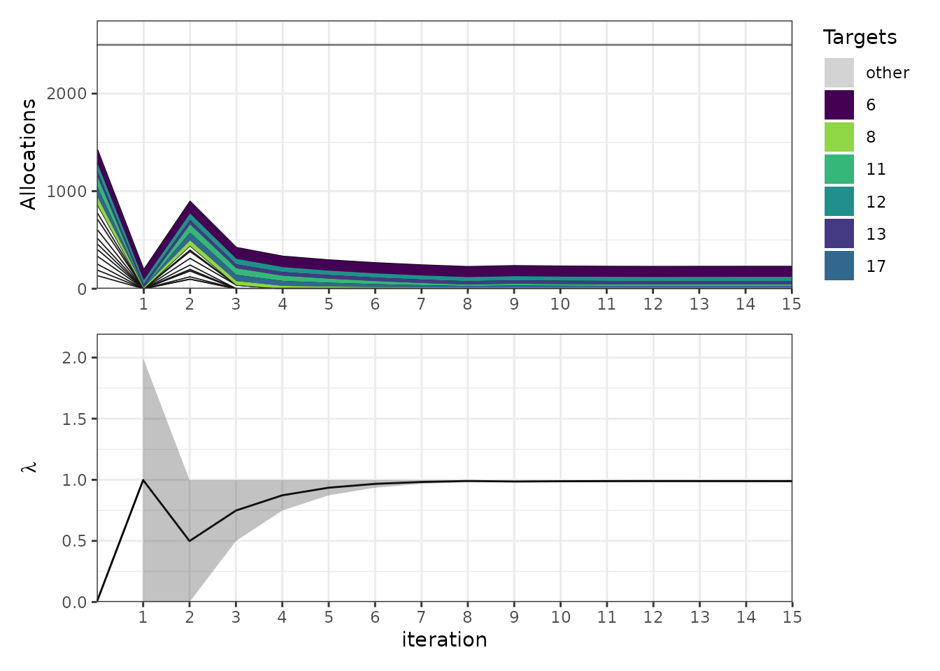

A bounded support

The second example uses Beta demand on $[x_{\min}, x_{\max}]$ rather than the whole real line. add_pdqr_funs() handles that with trans and trans_inv, which are composed onto the cdf and the quantile function respectively.

zxh_beta_forecasts <- zxh_tab3 |>
  mutate(stdize_news_params(ax = c, a_minus = v, a_plus = h), .after = c) |>
  as_tibble() |>
  rename(shape1 = Balpha, shape2 = Bbeta) |>
  add_pdqr_funs(
    types = c("p", "q"),
    dist = "beta",
    trans = function(x, x_min, x_max) (x - x_min) / (x_max - x_min),
    trans_inv = function(q, x_min, x_max) x_min + (x_max - x_min) * q
  )

allo_beta <- allocate(
  zxh_beta_forecasts,
  w = "c",
  K = 6500,
  target_names = "Product"
)

zxh_beta_forecasts |>
  select(Product, c, x_min, x_max, GIM, Opt) |>
  left_join(allo_beta$xdf[[1]], by = "Product") |>
  select(Product, c, x_min, x_max, GIM, Opt, ours = x) |>
  mutate(difference = ours - Opt)
#> # A tibble: 6 × 8
#>   Product     c x_min x_max   GIM   Opt  ours difference
#>   <chr>   <int> <int> <int> <dbl> <dbl> <dbl>      <dbl>
#> 1 1           4   100   300 207.  208.  208.   -0.00292 
#> 2 2           7    50   250  95.7  96.7  96.7  -0.00487 
#> 3 3          15    75   150  90.1  90.3  90.3  -0.000617
#> 4 4          10    50   200 100.  101.  101.   -0.00145 
#> 5 5          15    50   200  90.1  90.6  90.5  -0.000989
#> 6 6           6    73   275 209.  212.  212.   -0.000238

Every product is stocked here, and each allocation lands inside its own support.

beta_cmp <- zxh_beta_forecasts |>
  select(Product, c, Opt, x_min, x_max) |>
  left_join(allo_beta$xdf[[1]], by = "Product")
c(
  max_abs_difference = max(abs(beta_cmp$x - beta_cmp$Opt)),
  budget_spent = sum(beta_cmp$c * beta_cmp$x),
  budget_available = 6500,
  all_within_support = all(beta_cmp$x >= beta_cmp$x_min & beta_cmp$x <= beta_cmp$x_max)
)
#> max_abs_difference       budget_spent   budget_available all_within_support 
#>       4.867953e-03       6.500034e+03       6.500000e+03       1.000000e+00

Other parameterizations

Two more helpers convert application parameterizations into kappa and alpha: stdize_ou_params() takes explicit over- and under-prediction costs, and stdize_met_params() takes the cost-loss ratio used in the weather decision-analysis literature.

rbind(
  newsvendor = stdize_news_params(ax = 4, a_minus = 7, a_plus = 1),
  over_under = stdize_ou_params(O = 1, U = 3),
  cost_loss = stdize_met_params(C = 2, L = 10)
)
#>            kappa alpha
#> newsvendor     8 0.375
#> over_under     4 0.750
#> cost_loss     10 0.800

References

B. Zhang, X. Xu, and Z. Hua. “A binary solution method for the multiproduct newsboy problem with budget constraint.” International Journal of Production Economics, 117(1):136-141, 2009.

L. Abdel-Malek and R. Montanari. “An analysis of the multi-product newsboy problem with a budget constraint.” International Journal of Production Economics, 97(3):296-307, 2005.