distfromq
distfromq.RmdIntroduction
The distfromq package provides functions for
constructing an approximation to a probability distribution from a
finite set of quantiles of the distribution. The package provides four
main functions:
-
make_p_fnreturns a function that is analogous topnorm, and can be used to evaluate the approximated cumulative distribution function (CDF). -
make_d_fnreturns a function that is analogous todnorm, and can be used to evaluate the approximated probability density function (PDF). -
make_q_fnreturns a function that is analogous toqnorm, and can be used to evaluate the approximated quantile function (QF), i.e., the inverse CDF. -
make_r_fnreturns a function that is analogous tornorm, and can be used to simulate a pseudo-random sample from the approximated distribution.
All four functions take a set of probability levels (ps)
and the corresponding quantiles (qs) of the distribution to
be approximated as inputs, as well as arguments specifying the methods
for interpolating those quantiles to estimate the interior of the
distribution, and for extrapolating into the tails of the distribution
using a specified parametric family.
The next section of the vignette describes the methods that are used for approximating the distribution, and the following section gives examples.
Methods description
Suppose that we have a collection of pairs , , where for each , or for some distribution with CDF and quantile function . We allow for the distribution to have regions with no density or with discrete point masses, corresponding to regions where is flat or has a vertical step. In these instances, the points may fall within the flat region or partway up the vertical step, as will be illustrated below. Our goal is to reconstruct an estimate of , the corresponding PDF (if the distribution is continuous), and the QF , as well as a method for sampling from the distribution.
Our approach first splits the provided quantiles into a discrete part of the distribution and a continuous part. Then, for the continuous part it takes different strategies for interpolating on the interior of the provided quantiles and for extrapolating into the tails. We outline these procedures briefly here and give more detail below:
- Split into discrete and continuous parts.
- Discrete components of the distribution (i.e., point masses) are
identified in the following cases:
- there are repeated quantiles across different probability levels
(i.e.,
for some indices
).
In this case, we say that there is a point mass at the value(s) of
that was (were) repeated. The discrete distribution assigns probability
to each such point
corresponding to
.
The parameter
dup_tolcontrols identification of quantiles that are “close enough” to identify a point mass. - the parametric family to be used for extrapolation into the tails is
a lognormal distribution and there are one or more quantiles that are
approximately 0. In this case, we say that there is a point mass at
zero, with probability equal to
.
The parameter
zero_tolcontrols identification of quantiles that are “close enough to zero” to identify a point mass.
- there are repeated quantiles across different probability levels
(i.e.,
for some indices
).
In this case, we say that there is a point mass at the value(s) of
that was (were) repeated. The discrete distribution assigns probability
to each such point
corresponding to
.
The parameter
- The result of this step is a collection of locations of discrete point masses and their associated probabilities, and a set of quantiles and associated probability levels that can be used for estimating the continuous part of the distribution in the following step.
- Discrete components of the distribution (i.e., point masses) are
identified in the following cases:
- Estimate the continuous part of the distribution.
- On the interior of the quantiles for the continuous part of the distribution, we estimate the continuous component using a monotonic spline that interpolates the quantiles.
- We approximate the tails with a distribution in a specified location-scale family.
To estimate the quantile function (QF), we invert the estimate of the CDF. To estimate the probability density function (PDF), we use the derivative of the spline-based approximation to the CDF if there are no discrete components. This function does not support estimation of a density function if the distribution has any discrete components.
CDF estimation on the interior
The continuous distribution is estimated based on a set of adjusted quantile pairs that is obtained by eliminating duplicate quantiles, subtracting the cumulative probabilities associated with the discrete distribution, and renormalizing by the total probability mass associated with the discrete distribution. To approximate the CDF of the continuous distribution component at interior points, we fit a monotonic cubic Hermite spline that interpolates the set of “observations” (where these now denote the adjusted quantiles for the continuous distribution component). This spline fit yields a “stage 1” CDF estimate, .
To address issues with numerical stability in inverting the spline in the process of obtaining an estimate of the QF, we evaluate this stage 1 estimate at a grid of quantile values that are inserted between each consecutive pair of input quantiles (the number of new quantile values to use is an argument to the functions). We then use a “stage 2” CDF estimate that linearly interpolates this augmented grid of pairs. This behavior can be disabled if desired, though this is not recommended.
CDF estimation in the tails
We estimate the distribution for the left and right tails separately, assuming that they come from a specified location-scale family. The distributional family is assumed to be the same in each tail, but the location and scale parameters may differ in the left and right tails. Setting notation, suppose that where the random variable has a specified distribution. Recall that at the probability level , a quantile of can be calculated in terms of the corresponding quantile of via . Using the quantiles at two probability levels and , we can calculate the value of using
Similarly, we can calculate the value of as
In the above expressions, we use the two smallest quantiles when estimating the lower tail and the two largest quantiles when estimating the upper tail. With these choices, by construction the lower tail integrates to on the interval and the upper tail integrates to on the interval .
As an alternative, we also allow for the use of a log-normal distribution for extrapolation into the tails. The parameters of the log-normal distribution are estimated by applying the approach outlined above to the logarithms of the quantiles.
Estimation of the QF and PDF, and random deviate generation
To estimate the QF, we invert the CDF estimate, allowing for jumps in
regions where the CDF is flat. As noted above, this can be numerically
unstable if n_grid = NULL (thus using the spline fit
directly), so it is recommended that the n_grid parameter
be set to an integer if QF estimates are desired.
To estimate the PDF in instances where the CDF estimate corresponds to a continuous distribution, we differentiate the CDF estimate. If the stage 2 CDF estimate is used, this yields a “histogram density” estimate, which is discontinuous and piecewise constant. If this presents a challenge, the grid size can be increased or the stage 1 CDF estimate used instead.
Random deviates are obtained by sampling and then evaluating the approximated quantile function: .
Illustration of package functionality
We illustrate the package functionality with a series of four examples. The first example is a setting where the distribution is for a continuous random variable with a defined probability density function. The remaining examples illustrate the behavior of the functions in settings where the provided quantiles are the same at multiple probability levels or a lognormal distribution is used for tail extrapolation and there is at least one quantile at zero, indicating that there is some discrete component to the distribution.
library(distfromq)
library(ggplot2)
library(dplyr)
#>
#> Attaching package: 'dplyr'
#> The following objects are masked from 'package:stats':
#>
#>     filter, lag
#> The following objects are masked from 'package:base':
#>
#>     intersect, setdiff, setequal, union
Example 1
In our first example, we work with quantiles from the distribution . We compare this predictive distribution with three approximations of it that are derived from the quantiles using different assumptions for the tail behavior:
- The first assumes a log-normal distribution for the tails. This method should reconstruct the true distribution.
- The second assumes a normal distribution for the tails. This method has a mismatch in the support of the lower tail (including values less than 0), and has a thinner upper tail than the log-normal.
- The third assumes a Cauchy distribution for the tails. This method has a mismatch in the support of the lower tail (including values less than 0), and has a heavier upper tail than the log-normal.
quantile_probs <- seq(from = 0.1, to = 0.9, by = 0.1)

meanlog <- 4.0
sdlog <- 0.5
q_lognormal <- qlnorm(quantile_probs, meanlog = meanlog, sdlog = sdlog)
x <- seq(from = 0.0, to = 400.0, length = 501)
cdf_lognormal <- plnorm(x, meanlog = meanlog, sdlog = sdlog)

p_lognormal_approx <- make_p_fn(ps = quantile_probs,
                                qs = q_lognormal,
                                tail_dist = "lnorm")
cdf_lognormal_approx <- p_lognormal_approx(x)

# note that `tail_dist = "norm"` is the default; we specify it here for clarity
p_normal_approx <- make_p_fn(ps = quantile_probs,
                             qs = q_lognormal,
                             tail_dist = "norm")
cdf_normal_approx <- p_normal_approx(x)

p_cauchy_approx <- make_p_fn(ps = quantile_probs,
                             qs = q_lognormal,
                             tail_dist = "cauchy")
cdf_cauchy_approx <- p_cauchy_approx(x)

dplyr::bind_rows(
  data.frame(
    x = x,
    y = cdf_lognormal,
    dist = "Log normal"
  ),
  data.frame(
    x = x,
    y = cdf_lognormal_approx,
    dist = "Spline interpolation,\nlog-normal tails"
  ),
  data.frame(
    x = x,
    y = cdf_normal_approx,
    dist = "Spline interpolation,\nnormal tails"
  ),
  data.frame(
    x = x,
    y = cdf_cauchy_approx,
    dist = "Spline interpolation,\nCauchy tails"
  )
) %>%
  ggplot() +
  geom_line(
    mapping = aes(x = x, y = y, color = dist, linetype = dist),
    size = 0.8
  ) +
  geom_point(
    data = data.frame(q = q_lognormal, p = quantile_probs),
    mapping = aes(x = q, y = p),
    size = 1.2
  ) +
  scale_color_viridis_d(
    "Distribution",
    end = 0.9
  ) +
  scale_linetype_discrete("Distribution") +
  ylab("Probability") +
  xlab("") +
  theme_bw()
#> Warning: Using `size` aesthetic for lines was deprecated in ggplot2 3.4.0.
#> ℹ Please use `linewidth` instead.
#> This warning is displayed once every 8 hours.
#> Call `lifecycle::last_lifecycle_warnings()` to see where this warning was
#> generated.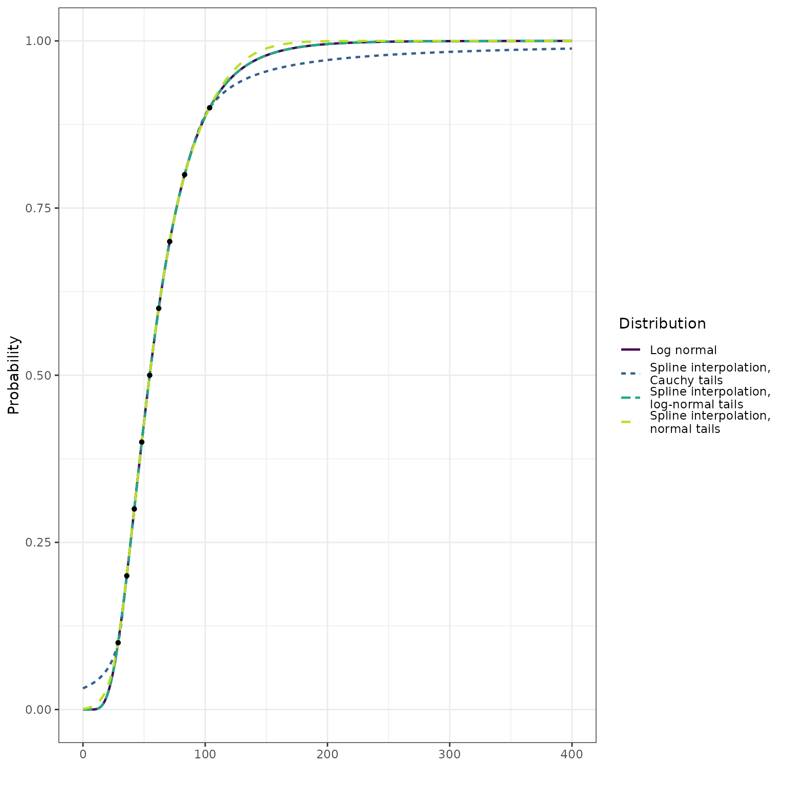
The following illustrates differences in the density estimates.
d_lognormal_approx <- make_d_fn(ps = quantile_probs,
                                qs = q_lognormal,
                                tail_dist = "lnorm")

d_normal_approx <- make_d_fn(ps = quantile_probs,
                             qs = q_lognormal,
                             tail_dist = "norm")

d_cauchy_approx <- make_d_fn(ps = quantile_probs,
                             qs = q_lognormal,
                             tail_dist = "cauchy")

pdf_lognormal <- dlnorm(x, meanlog = meanlog, sdlog = sdlog)
pdf_lognormal_approx <- d_lognormal_approx(x)
pdf_normal_approx <- d_normal_approx(x)
pdf_cauchy_approx <- d_cauchy_approx(x)

dplyr::bind_rows(
  data.frame(
    x = x,
    y = pdf_lognormal,
    dist = "Log normal"
  ),
  data.frame(
    x = x,
    y = pdf_lognormal_approx,
    dist = "Spline interpolation,\nlog-normal tails"
  ),
  data.frame(
    x = x,
    y = pdf_normal_approx,
    dist = "Spline interpolation,\nnormal tails"
  ),
  data.frame(
    x = x,
    y = pdf_cauchy_approx,
    dist = "Spline interpolation,\nCauchy tails"
  )
) %>%
  ggplot() +
  geom_vline(
    data = data.frame(q = q_lognormal),
    mapping = aes(xintercept = q),
    size = 0.2
  ) +
  geom_line(
    mapping = aes(x = x, y = y, color = dist, linetype = dist),
    size = 0.8
  ) +
  scale_color_viridis_d(
    "Distribution",
    end = 0.9
  ) +
  scale_linetype_discrete("Distribution") +
  ylab("Probability Density") +
  xlab("") +
  theme_bw()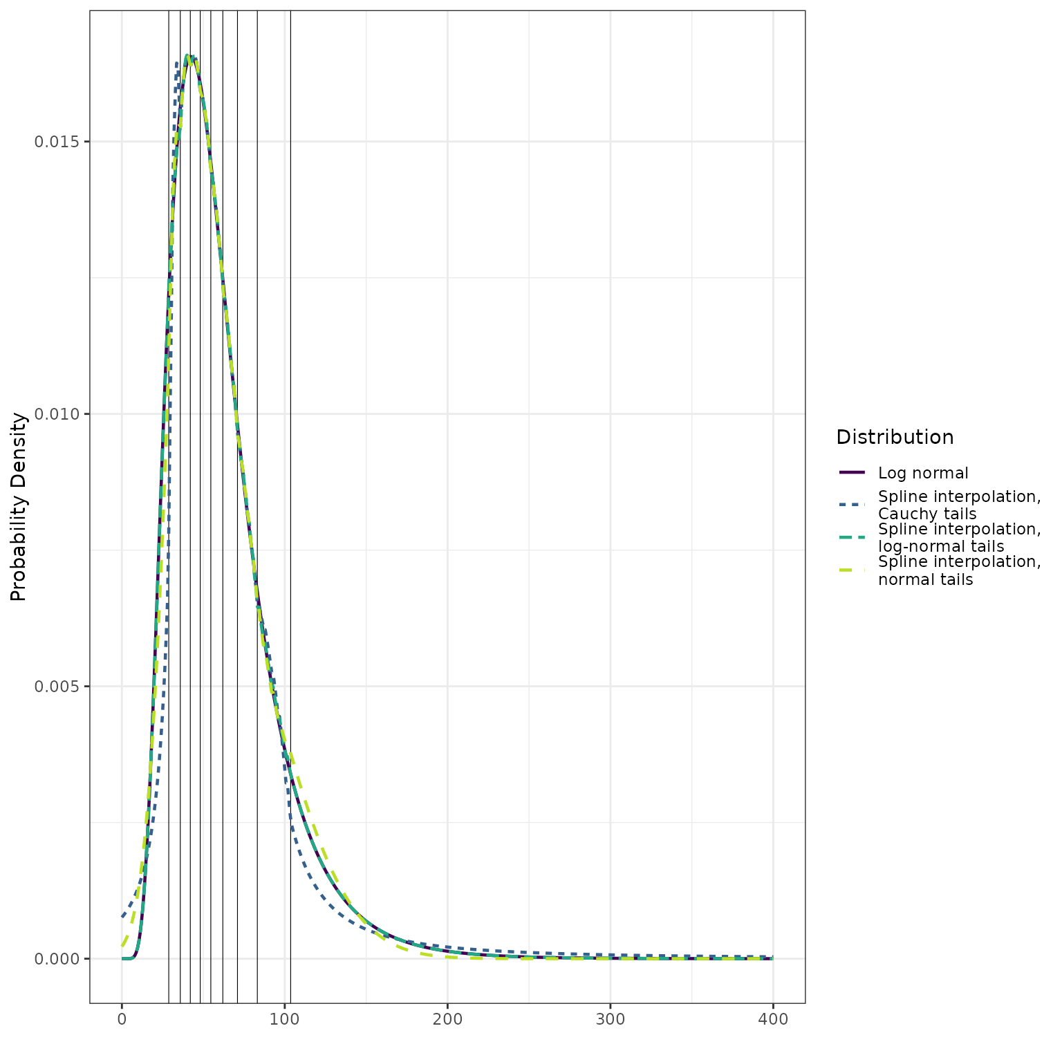
We emphasize that the density is a step function. We illustrate this
by setting the n_grid parameter to the artificially low
value of 1:
d_lognormal_approx_n_grid_1 <- make_d_fn(ps = quantile_probs,
                                         qs = q_lognormal,
                                         tail_dist = "lnorm",
                                         interior_args = list(n_grid = 1))

pdf_lognormal_approx_n_grid_1 <- d_lognormal_approx_n_grid_1(x)

dplyr::bind_rows(
  data.frame(
    x = x,
    y = pdf_lognormal_approx,
    dist = "Spline interpolation,\n n_grid = 20"
  ),
  data.frame(
    x = x,
    y = pdf_lognormal_approx_n_grid_1,
    dist = "Spline interpolation,\n n_grid = 1"
  )
) %>%
  ggplot() +
  geom_vline(
    data = data.frame(q = q_lognormal),
    mapping = aes(xintercept = q),
    size = 0.2
  ) +
  geom_line(
    mapping = aes(x = x, y = y, color = dist),
    size = 0.8
  ) +
  scale_color_viridis_d(
    "Distribution",
    end = 0.7
  ) +
  scale_linetype_discrete("Distribution") +
  ylab("Probability Density") +
  xlab("") +
  theme_bw()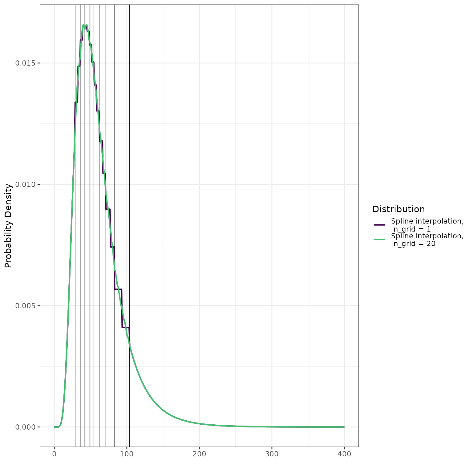
We can generate random deviates from the distribution estimates as follows:
r_normal_approx <- make_r_fn(ps = quantile_probs,
                             qs = q_lognormal,
                             tail_dist = "norm")
r_lognormal_approx <- make_r_fn(ps = quantile_probs,
                                qs = q_lognormal,
                                tail_dist = "lnorm")
r_cauchy_approx <- make_r_fn(ps = quantile_probs,
                             qs = q_lognormal,
                             tail_dist = "cauchy")

normal_approx_sample <- r_normal_approx(n = 10000)
lognormal_approx_sample <- r_lognormal_approx(n = 10000)
cauchy_approx_sample <- r_cauchy_approx(n = 10000)

bind_rows(
  data.frame(x = normal_approx_sample, dist = "Spline interpolation,\nnormal tails"),
  data.frame(x = lognormal_approx_sample, dist = "Spline interpolation,\nlog-normal tails"),
  data.frame(x = cauchy_approx_sample, dist = "Spline interpolation,\nCauchy tails")
) %>%
  ggplot() +
  geom_density(mapping = aes(x = x, color = dist, linetype = dist)) +
  scale_color_viridis_d(
    "Distribution",
    end = 0.9
  ) +
  scale_linetype_discrete("Distribution") +
  theme_bw()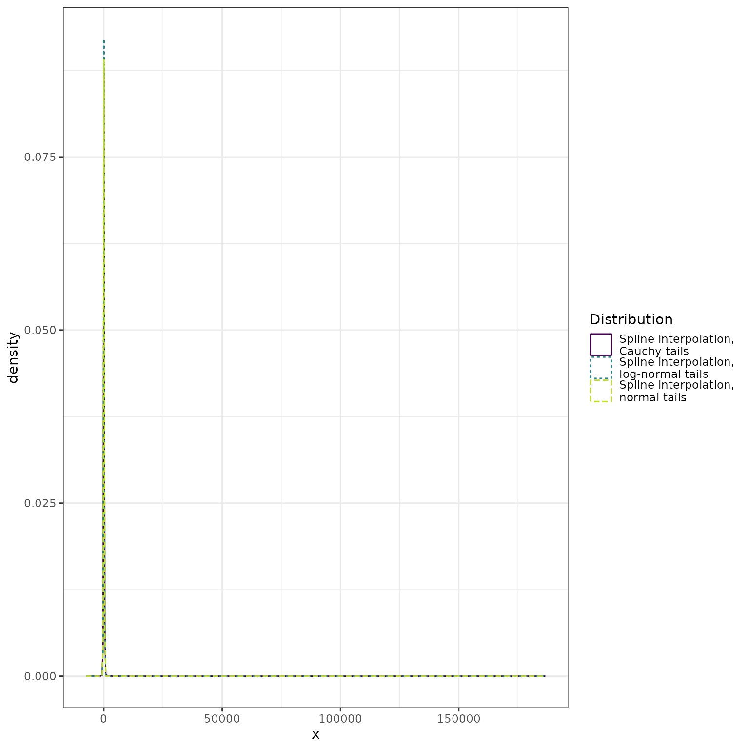
The heavy tails of the Cauchy distribution dominate the display. Here we restrict the range of the horizontal axis:
bind_rows(
  data.frame(x = normal_approx_sample, dist = "Spline interpolation,\nnormal tails"),
  data.frame(x = lognormal_approx_sample, dist = "Spline interpolation,\nlog-normal tails"),
  data.frame(x = cauchy_approx_sample, dist = "Spline interpolation,\nCauchy tails")
) %>%
  ggplot() +
  geom_density(mapping = aes(x = x, color = dist, linetype = dist)) +
  scale_color_viridis_d(
    "Distribution",
    end = 0.9
  ) +
  scale_linetype_discrete("Distribution") +
  xlim(-100, 300) +
  theme_bw()
#> Warning: Removed 280 rows containing non-finite outside the scale range
#> (`stat_density()`).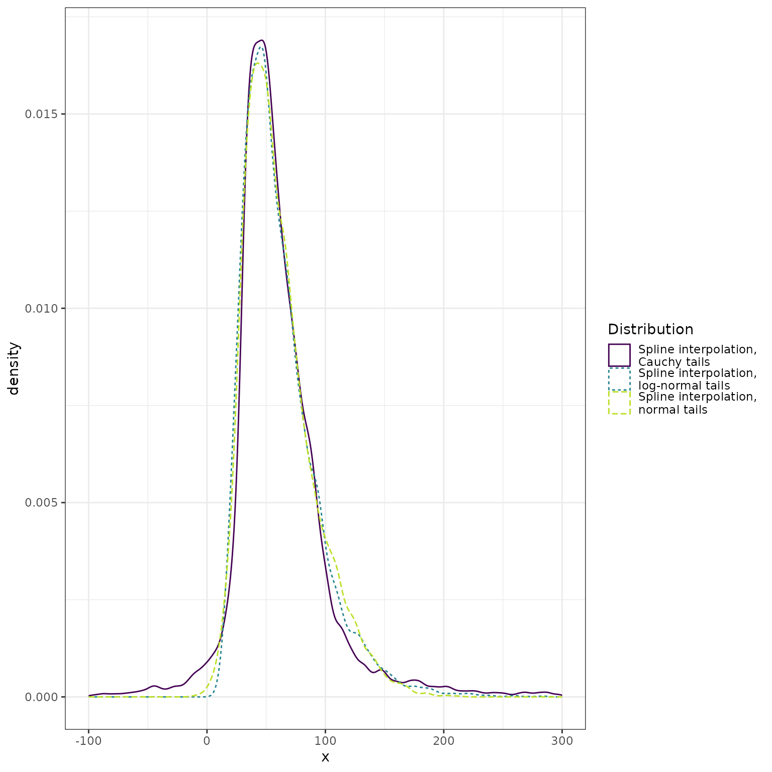
Finally, we display quantile function estimates:
ps <- seq(from = 0.01, to = 0.99, by = 0.01)

q_normal_approx <- make_q_fn(ps = quantile_probs,
                             qs = q_lognormal,
                             tail_dist = "norm")
q_lognormal_approx <- make_q_fn(ps = quantile_probs,
                                qs = q_lognormal,
                                tail_dist = "lnorm")
q_cauchy_approx <- make_q_fn(ps = quantile_probs,
                             qs = q_lognormal,
                             tail_dist = "cauchy")

quantiles_lognormal <- qlnorm(ps, meanlog = meanlog, sdlog = sdlog)
quantiles_normal_approx <- q_normal_approx(ps)
quantiles_lognormal_approx <- q_lognormal_approx(ps)
quantiles_cauchy_approx <- q_cauchy_approx(ps)


dplyr::bind_rows(
  data.frame(
    x = ps,
    y = quantiles_lognormal,
    dist = "Log normal"
  ),
  data.frame(
    x = ps,
    y = quantiles_normal_approx,
    dist = "Spline interpolation,\nnormal tails"
  ),
  data.frame(
    x = ps,
    y = quantiles_lognormal_approx,
    dist = "Spline interpolation,\nlognormal tails"
  ),
  data.frame(
    x = ps,
    y = quantiles_cauchy_approx,
    dist = "Spline interpolation,\nCauchy tails"
  )
) %>%
  ggplot() +
  geom_line(
    mapping = aes(x = x, y = y, color = dist, linetype = dist),
    size = 0.8
  ) +
  scale_color_viridis_d(
    "Distribution",
    end = 0.9
  ) +
  scale_linetype_discrete("Distribution") +
  ylab("Quantile") +
  xlab("Probability Level") +
  theme_bw()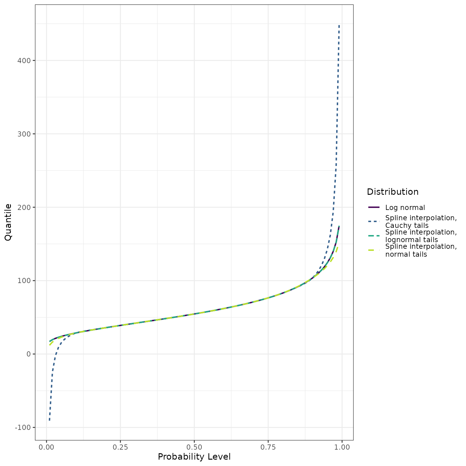
Example 2: lognormal tails with a point mass at 0
A lognormal distribution specifies that , i.e., the random variable will always non-negative values. If a lognormal tail distribution is used, e.g. to ensure that the distribution’s support is non-negative and to capture a long right tail, the package inserts a point mass at 0 if any provided quantiles are 0. We illustrate this behavior in this example.
# mixture of a LogNormal(4, 0.5) distribution with weight 0.8 and
# a point mass at 0 with weight 0.2

# probabilities and quantiles for the lognormal component
lnorm_ps <- seq(from = 0.1, to = 0.9, by = 0.1)
lnorm_qs <- qlnorm(lnorm_ps, meanlog = 4.0, sdlog = 0.5)
adj_lnorm_ps <- 0.2 + lnorm_ps * 0.8

# quantile at 0 with probability 0.2 for the point mass at 0
point_p <- 0.2
point_q <- 0.0

ps <- c(point_p, adj_lnorm_ps)
qs <- c(point_q, lnorm_qs)
Note that the CDF estimate is zero below 0, jumps to 0.2 at 0, and is continuous thereafter.
x <- seq(from = -100.0, to = 400.0, length = 501)

p_lognormal_approx <- make_p_fn(ps = ps,
                                qs = qs,
                                tail_dist = "lnorm")
cdf_lognormal_approx <- p_lognormal_approx(x)

data.frame(
  x = x,
  y = cdf_lognormal_approx
) %>%
  ggplot() +
  geom_line(
    mapping = aes(x = x, y = y),
    size = 0.8
  ) +
  geom_point(
    data = data.frame(q = qs, p = ps),
    mapping = aes(x = q, y = p),
    size = 1.2
  ) +
  ylim(0, 1) +
  ylab("Probability") +
  xlab("") +
  theme_bw()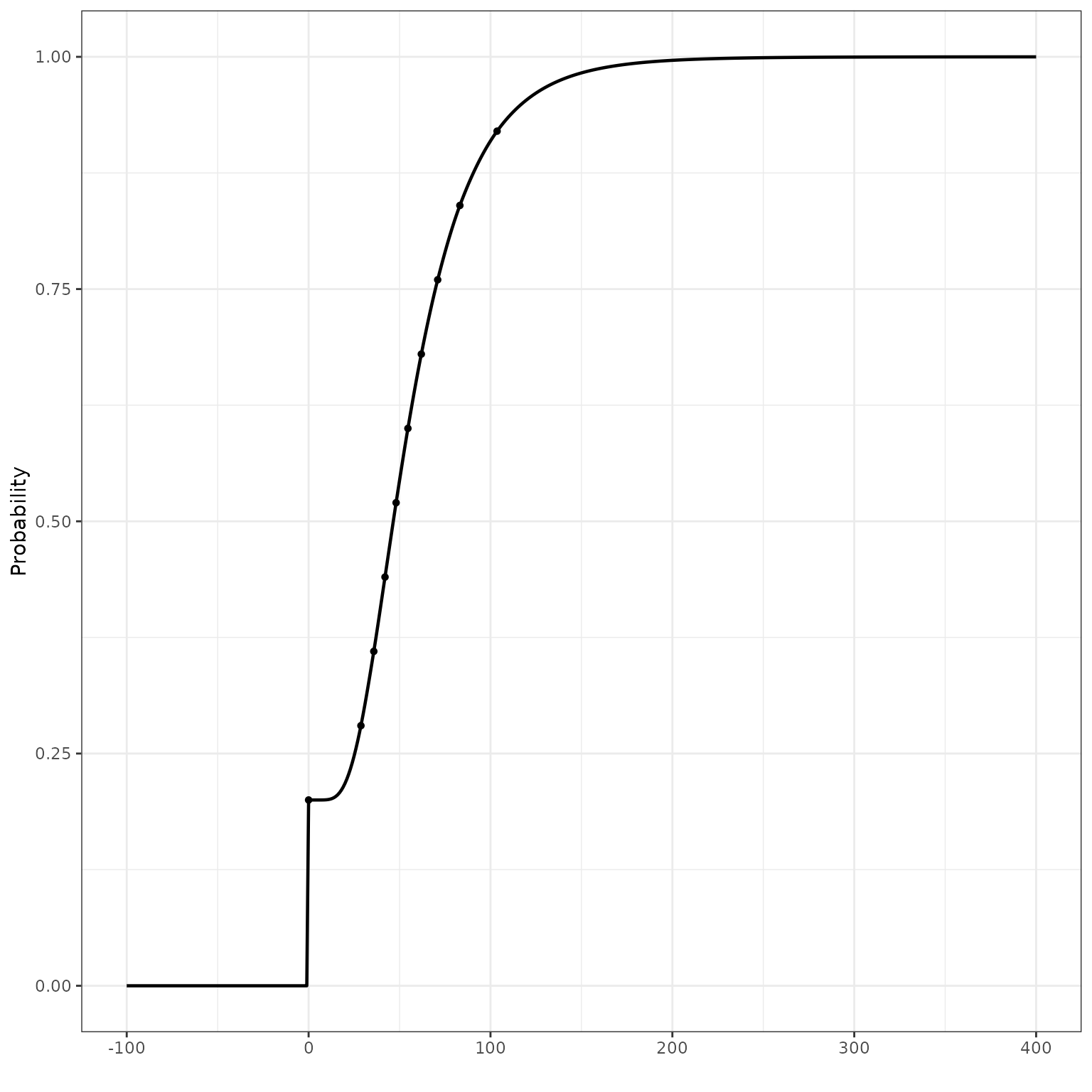
As expected, the quantile function inverts the CDF.
plot_ps <- seq(from = 0.00, to = 0.99, by = 0.001)

q_lognormal_approx <- make_q_fn(ps = ps,
                                qs = qs,
                                tail_dist = "lnorm")
qf_lognormal_approx <- q_lognormal_approx(plot_ps)

data.frame(
  x = plot_ps,
  y = qf_lognormal_approx
) %>%
  ggplot() +
  geom_line(
    mapping = aes(x = x, y = y),
    size = 0.8
  ) +
  geom_point(
    data = data.frame(q = ps, p = qs),
    mapping = aes(x = q, y = p),
    size = 1.2
  ) +
  xlim(0, 1) +
  xlab("Probability") +
  ylab("") +
  theme_bw()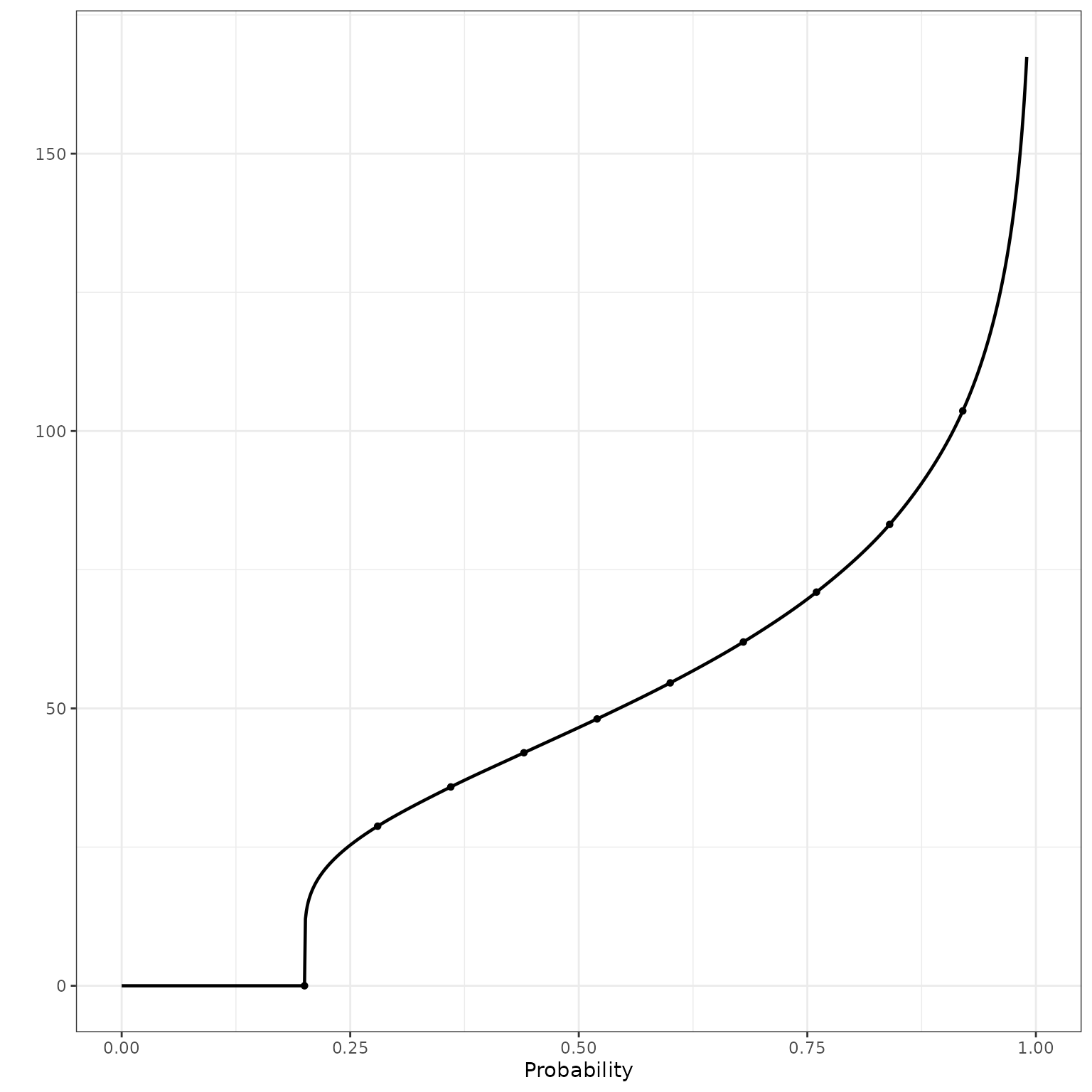
We can verify this by plotting the quantile function estimate with inverted axes on the same display as the CDF estimate:
dplyr::bind_rows(
  data.frame(
    x = x,
    y = cdf_lognormal_approx,
    method = "CDF Estimate"
  ),
  data.frame(
    x = qf_lognormal_approx,
    y = plot_ps,
    method = "Flipped QF Estimate"
  )
) %>%
  ggplot() +
  geom_line(
    mapping = aes(x = x, y = y, color = method, linetype = method),
    size = 0.8
  ) +
  geom_point(
    data = data.frame(q = qs, p = ps),
    mapping = aes(x = q, y = p),
    size = 1.2
  ) +
  ylim(0, 1) +
  ylab("Probability") +
  xlab("") +
  theme_bw()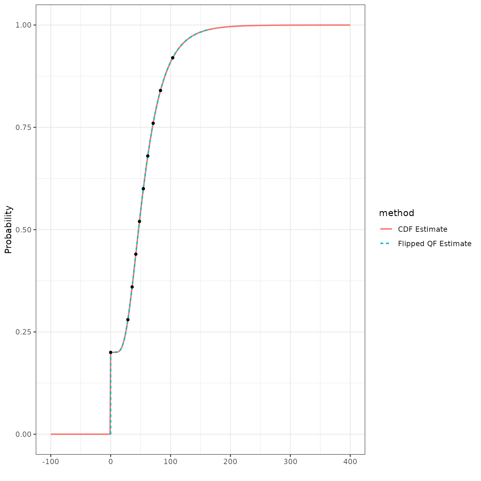
Samples from this distribution estimate will include a concentration of values at 0:
r_fn <- make_r_fn(ps = ps, qs = qs, tail_dist = "lnorm")

sampled_values_df <- data.frame(x = r_fn(10000))

ggplot(sampled_values_df) +
  geom_histogram(mapping = aes(x = x), bins = 100) +
  theme_bw()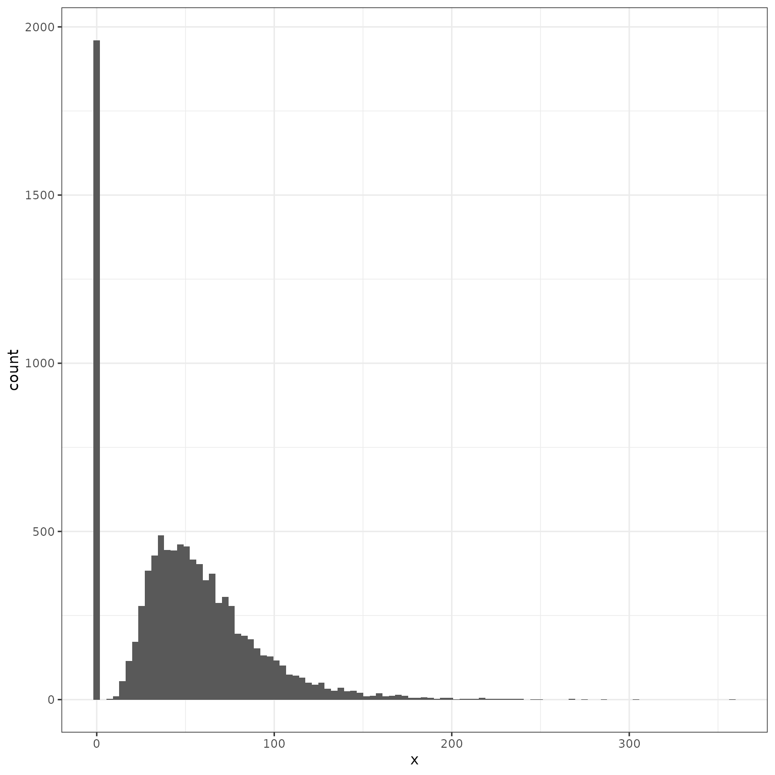
mean(sampled_values_df$x == 0)
#> [1] 0.196
Because the distribution has a discrete component, we cannot produce a density estimate:
d_fn_lnorm <- make_d_fn(ps = ps, qs = qs, tail_dist = "lnorm")
#> Error in make_d_fn(ps = ps, qs = qs, tail_dist = "lnorm"): make_d_fn requires the distribution to be continuous, but a discrete component was detected
Note that we do not get an error when estimating the density with a normal tail distribution, because in this case we are not forced to assume that there is a point mass at 0:
d_fn_norm <- make_d_fn(ps = ps, qs = qs, tail_dist = "norm")Example 3: duplicated quantiles on the interior
When quantile values are the same at multiple probability levels, the
distribution assigns non-zero probability to that value, corresponding
to a “step” or “jump” in the cumulative distribution function. Again, we
note that in this case, make_d_fn will throw an error
because a continuous density does not exist. We illustrate the behavior
of the estimates provided by make_p_fn and
make_q_fn in the presence of repeated quantiles in this and
the following example.
quantile_probs <- seq(from = 0.1, to = 0.9, by = 0.1)
quantile_values <- c(1.0, 2.0, 3.0, 3.0, 3.0, 3.0, 3.0, 8.0, 9.0)

d_normal_approx <- make_d_fn(ps = quantile_probs,
                             qs = quantile_values,
                             tail_dist = "norm")
#> Error in make_d_fn(ps = quantile_probs, qs = quantile_values, tail_dist = "norm"): make_d_fn requires the distribution to be continuous, but a discrete component was detected
p_normal_approx <- make_p_fn(ps = quantile_probs,
                             qs = quantile_values,
                             tail_dist = "norm")
q_normal_approx <- make_q_fn(ps = quantile_probs,
                             qs = quantile_values,
                             tail_dist = "norm")
r_normal_approx <- make_r_fn(ps = quantile_probs,
                             qs = quantile_values,
                             tail_dist = "norm")

x <- seq(from = 0.0, to = 20.0, length = 5001)
cdf_normal_approx <- p_normal_approx(x)
ggplot() +
  geom_line(data = data.frame(x = x, y = cdf_normal_approx),
            mapping = aes(x = x, y = y)) +
  geom_point(data = data.frame(x = quantile_values, y = quantile_probs),
             mapping = aes(x = x, y = y))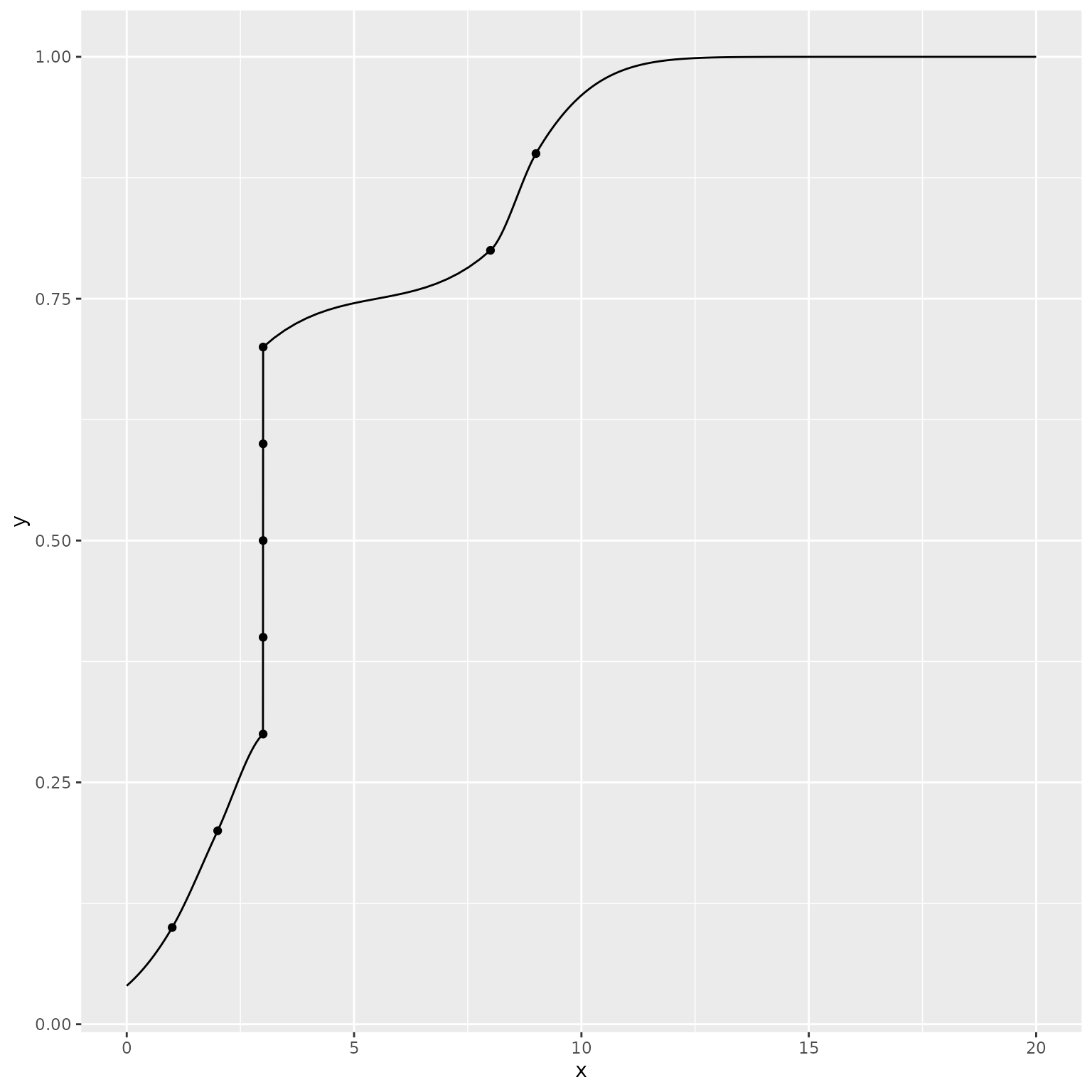
ps <- seq(from = 0.0, to = 1.0, length = 5001)
qf_normal_approx <- q_normal_approx(ps)
ggplot() +
  geom_line(data = data.frame(p = ps, y = qf_normal_approx),
            mapping = aes(x = p, y = y)) +
  geom_point(data = data.frame(x = quantile_probs, y = quantile_values),
             mapping = aes(x = x, y = y))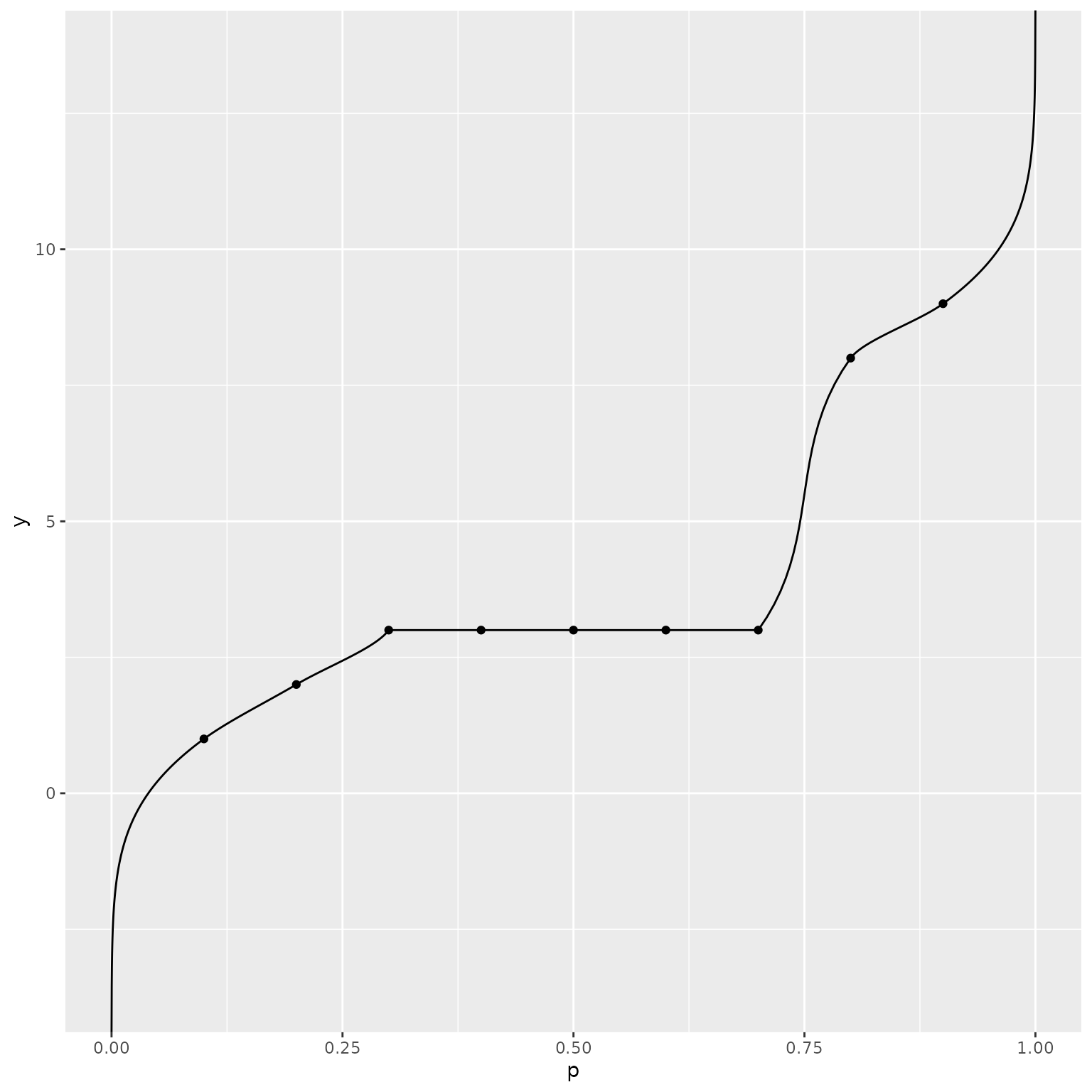
samples_normal_approx <- r_normal_approx(n = 10000)
mean(samples_normal_approx == 3.0)
#> [1] 0.3994
We confirm here that the estimated CDF and QF are indeed inverses to a high degree of numerical precision in regions where the distribution is continuous:
ps <- seq(from = 0.0, to = 1.0, length = 101)
out_ps <- p_normal_approx(q_normal_approx(ps))
out_ps
#>   [1] 0.00 0.01 0.02 0.03 0.04 0.05 0.06 0.07 0.08 0.09 0.10 0.11 0.12 0.13 0.14
#>  [16] 0.15 0.16 0.17 0.18 0.19 0.20 0.21 0.22 0.23 0.24 0.25 0.26 0.27 0.28 0.29
#>  [31] 0.30 0.70 0.70 0.70 0.70 0.70 0.70 0.70 0.70 0.70 0.70 0.70 0.70 0.70 0.70
#>  [46] 0.70 0.70 0.70 0.70 0.70 0.70 0.70 0.70 0.70 0.70 0.70 0.70 0.70 0.70 0.70
#>  [61] 0.70 0.70 0.70 0.70 0.70 0.70 0.70 0.70 0.70 0.70 0.70 0.71 0.72 0.73 0.74
#>  [76] 0.75 0.76 0.77 0.78 0.79 0.80 0.81 0.82 0.83 0.84 0.85 0.86 0.87 0.88 0.89
#>  [91] 0.90 0.91 0.92 0.93 0.94 0.95 0.96 0.97 0.98 0.99 1.00

ps[(ps < 0.3) | (ps > 0.7)] - out_ps[(ps < 0.3) | (ps > 0.7)]
#>  [1]  0.000000e+00 -1.561251e-17 -3.469447e-18 -1.040834e-17  0.000000e+00
#>  [6] -2.775558e-17  2.775558e-17  0.000000e+00  0.000000e+00  0.000000e+00
#> [11]  0.000000e+00  0.000000e+00  0.000000e+00  0.000000e+00  0.000000e+00
#> [16]  0.000000e+00  0.000000e+00  0.000000e+00  0.000000e+00 -2.775558e-17
#> [21]  0.000000e+00  0.000000e+00  2.775558e-17  0.000000e+00  0.000000e+00
#> [26]  0.000000e+00  5.551115e-17  0.000000e+00  0.000000e+00  0.000000e+00
#> [31]  0.000000e+00  0.000000e+00  0.000000e+00  0.000000e+00  0.000000e+00
#> [36]  0.000000e+00  0.000000e+00  0.000000e+00  0.000000e+00  0.000000e+00
#> [41]  0.000000e+00  0.000000e+00  0.000000e+00  0.000000e+00  1.110223e-16
#> [46]  0.000000e+00  0.000000e+00 -1.110223e-16  0.000000e+00 -1.110223e-16
#> [51]  0.000000e+00  0.000000e+00  1.110223e-16  0.000000e+00  0.000000e+00
#> [56]  0.000000e+00  0.000000e+00  1.110223e-16  0.000000e+00  0.000000e+00
#> [61]  0.000000e+00
As described earlier, we use a piecewise linear representation of the
CDF to avoid numerical issues that arise when inverting the monotonic
spline. We illustrate these problems by manually setting
n_grid = NULL, i.e., using the stage 1 CDF estimate based
directly on splines. The two representations of the CDF are generally
quite similar, but the QF estimates can differ substantially.
p_normal_approx_spline <- make_p_fn(ps = quantile_probs,
                                    qs = quantile_values,
                                    tail_dist = "norm",
                                    interior_args = list(n_grid = NULL))
q_normal_approx_spline <- make_q_fn(ps = quantile_probs,
                                    qs = quantile_values,
                                    tail_dist = "norm",
                                    interior_args = list(n_grid = NULL))

x <- seq(from = 0.0, to = 20.0, length = 5001)
plot_df <- rbind(
  data.frame(
    x = x,
    cdf = p_normal_approx(x),
    type = "piecewise linear"
  ),
  data.frame(
    x = x,
    cdf = p_normal_approx_spline(x),
    type = "spline"
  )
)
ggplot() +
  geom_line(data = plot_df,
            mapping = aes(x = x, y = cdf, color = type, linetype = type)) +
  geom_point(data = data.frame(x = quantile_values, y = quantile_probs),
             mapping = aes(x = x, y = y))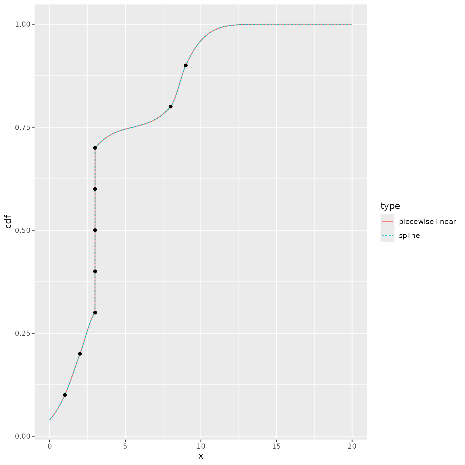
ps <- seq(from = 0.0, to = 1.0, length = 5001)
plot_df <- rbind(
  data.frame(
    p = ps,
    qf = q_normal_approx(ps),
    type = "piecewise linear"
  ),
  data.frame(
    p = ps,
    qf = q_normal_approx_spline(ps),
    type = "spline"
  )
)
ggplot() +
  geom_line(data = plot_df,
            mapping = aes(x = p, y = qf, color = type, linetype = type)) +
  geom_point(data = data.frame(x = quantile_probs, y = quantile_values),
             mapping = aes(x = x, y = y))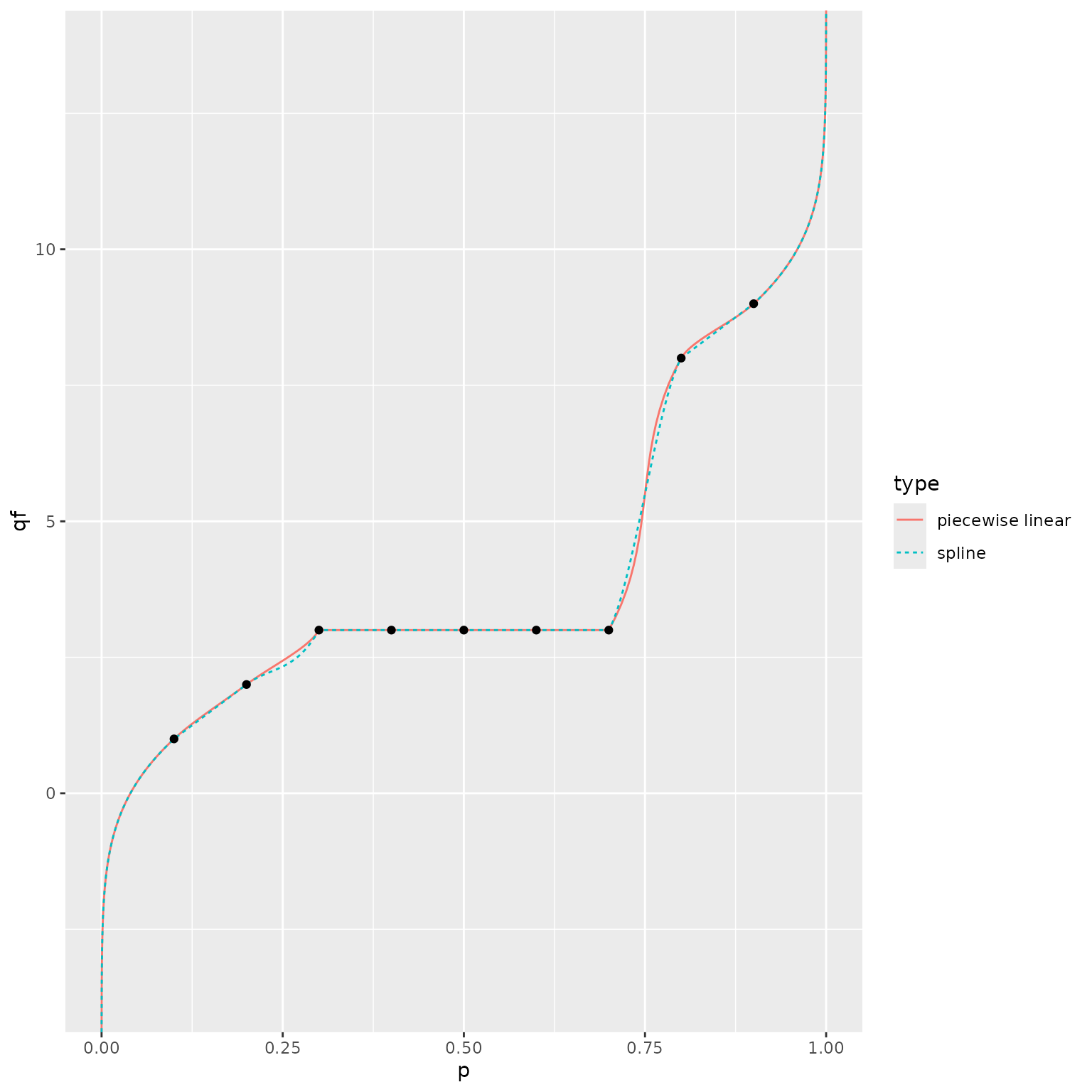
We therefore recommend using the piecewise linear representation when using a quantile function or generating random deviates, which uses the quantile function in the background.
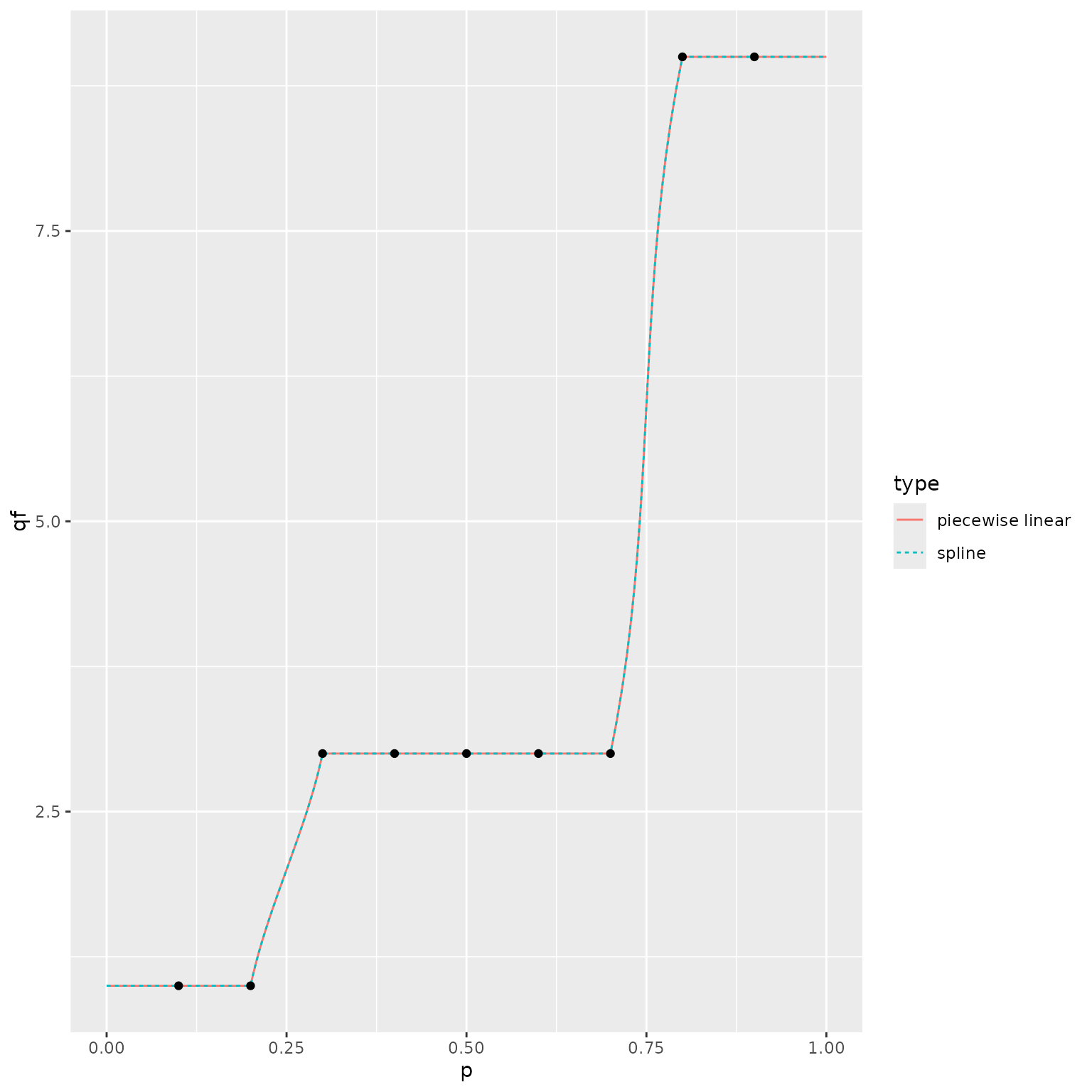
Example 4: duplicated quantiles in the tails
Our final example illustrates the behavior when there are duplicated
quantiles at the edges. In these cases, we ignore the specified
tail_dist, and assume that the point mass at the edge
contains all of the tail probability.
quantile_probs <- seq(from = 0.1, to = 0.9, by = 0.1)
quantile_values <- c(1.0, 1.0, 3.0, 3.0, 3.0, 3.0, 3.0, 9.0, 9.0)

p_normal_approx <- make_p_fn(ps = quantile_probs,
                             qs = quantile_values,
                             tail_dist = "norm")
p_normal_approx_lin <- make_p_fn(ps = quantile_probs,
                                 qs = quantile_values,
                                 tail_dist = "norm",
                                 interior_args = list(n_grid = 20))
q_normal_approx <- make_q_fn(ps = quantile_probs,
                             qs = quantile_values,
                             tail_dist = "norm")
q_normal_approx_lin <- make_q_fn(ps = quantile_probs,
                                 qs = quantile_values,
                                 tail_dist = "norm",
                                 interior_args = list(n_grid = 20))

x <- seq(from = 0.0, to = 20.0, length = 5001)
plot_df <- rbind(
  data.frame(
    x = x,
    cdf = p_normal_approx(x),
    type = "spline"
  ),
  data.frame(
    x = x,
    cdf = p_normal_approx_lin(x),
    type = "piecewise linear"
  )
)
ggplot() +
  geom_line(data = plot_df,
            mapping = aes(x = x, y = cdf, color = type, linetype = type)) +
  geom_point(data = data.frame(x = quantile_values, y = quantile_probs),
             mapping = aes(x = x, y = y))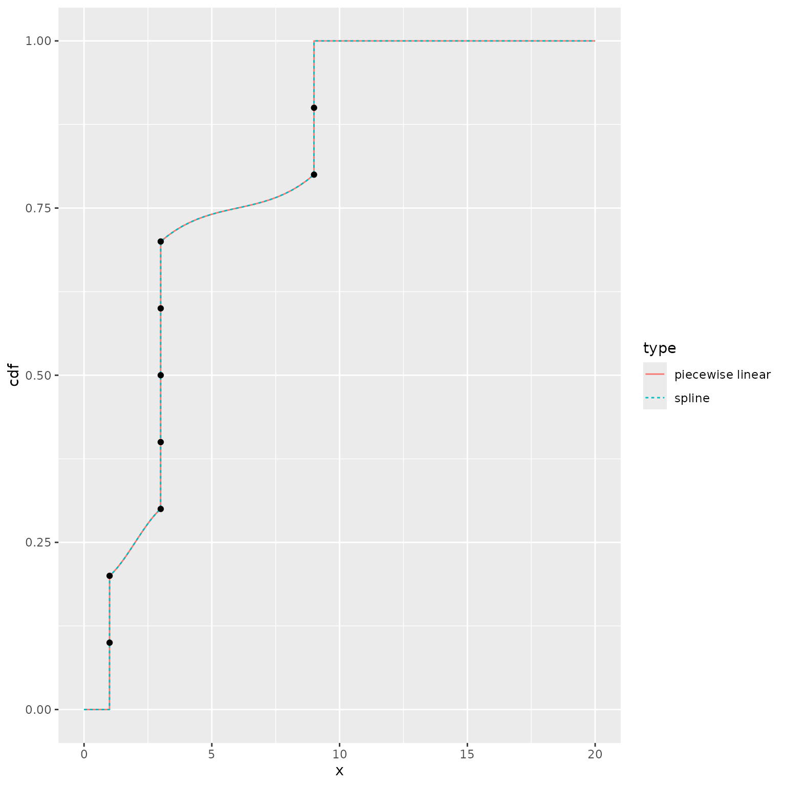
ps <- seq(from = 0.0, to = 1.0, length = 5001)
plot_df <- rbind(
  data.frame(
    p = ps,
    qf = q_normal_approx(ps),
    type = "spline"
  ),
  data.frame(
    p = ps,
    qf = q_normal_approx_lin(ps),
    type = "piecewise linear"
  )
)
ggplot() +
  geom_line(data = plot_df,
            mapping = aes(x = p, y = qf, color = type, linetype = type)) +
  geom_point(data = data.frame(x = quantile_probs, y = quantile_values),
             mapping = aes(x = x, y = y))