About ForecastFramework

Purpose

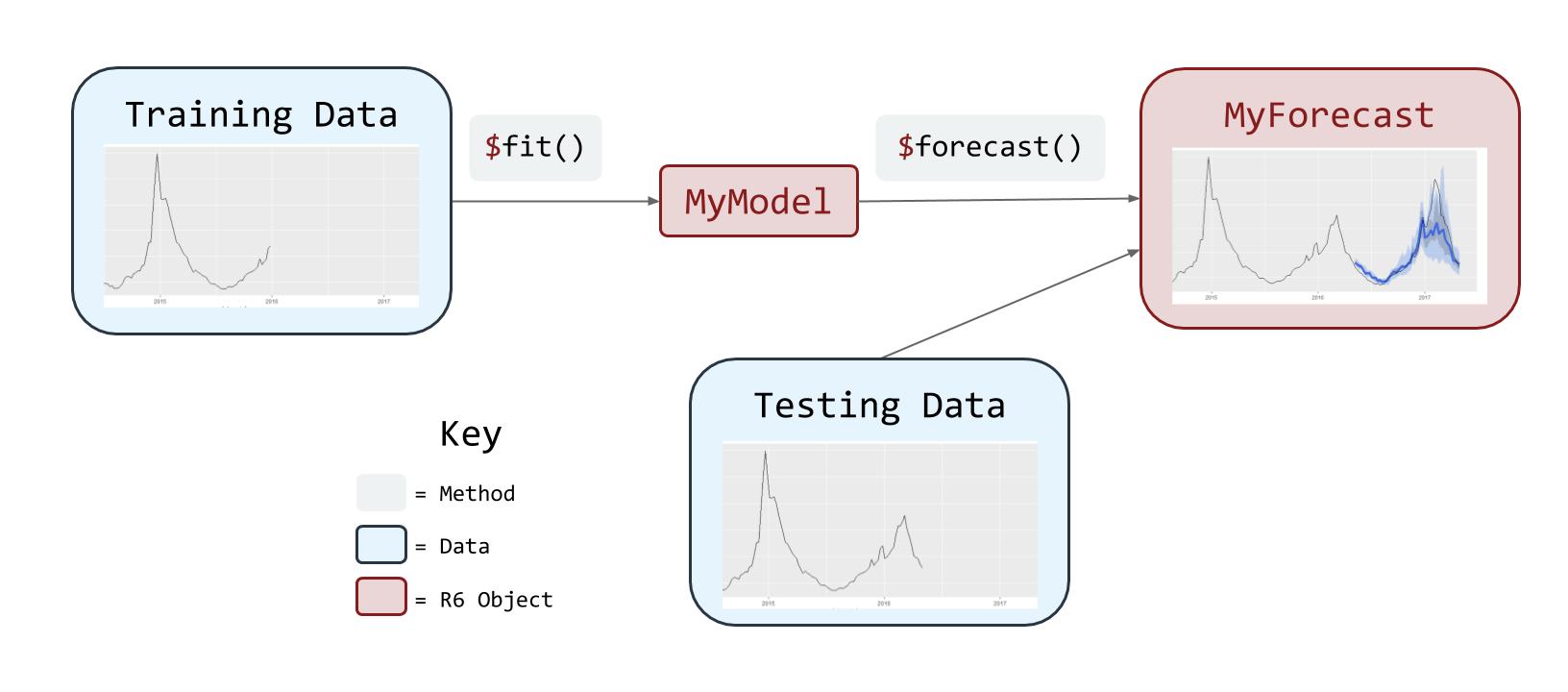
ForecastFramework is an object-oriented R package that standardizes forecasting models. The package uses the R6 class implementation to design an object-oriented framework for building forecasting models for spatial time-series data. The central goals of the ForecastFramework package are to enable rapid model development while standardizing and simplifying implementation and performance evaluation.

Usage

ForecastFramework is one of the primary forecast modeling tools used at the Reich Lab at the University of Massachusetts Amherst. As one example, we use it under the hood in generating our real-time dengue forecasts for the Ministry of Public Health in Thailand.

The following diagram illustrates the flow of a ForecastFramework Modeling process:

Creation

ForecastFramework was created by Joshua Kaminsky of the Infectious Disease Dynamics Group at Johns Hopkins University. This demo was created by Katie House.

Getting Started

Installation of Forecast Framework

ForecastFramework is an open source R package hosted on CRAN and Github.

To install this package, run either of the following commands in your Rstudio console:

library(devtools)
devtools::install_github('HopkinsIDD/ForecastFramework')

Run this to ensure you have all the Dependencies

Run these lines of code before performing the vignette. NOTE: you only need to run this once. This script installs all of the necessary R packages for the rest of the demo.

install.packages(c('R6','devtools','forecast','ggplot2',
                   'gridExtra','data.table','knitr','kableExtra','RCurl'))
install.packages("dplyr", repos = "https://cloud.r-project.org")

Then run these commands:

library(devtools)
devtools::install_github('HopkinsIDD/ForecastFramework')
devtools::install_github('reichlab/sarimaTD') 
devtools::install_github("hrbrmstr/cdcfluview")

Test your packages are correctly installed with these commands:

# Forecast Framework Dependencies
library(ForecastFramework)
library(R6)
library(forecast)

# Data Dependencies
library(cdcfluview)
library(dplyr)
library(ggplot2)
library(gridExtra)
library(data.table)
library(knitr)
library(kableExtra)

# Function of Source Github Models
source_github <- function(u) {
  library(RCurl)
  # read script lines from website and evaluate
  script <- getURL(u, ssl.verifypeer = FALSE)
  eval(parse(text = script),envir=.GlobalEnv)
}  
# Source R6 Files
source_github('https://raw.githubusercontent.com/reichlab/forecast-framework-demos/master/models/ContestModel.R')
source_github('https://raw.githubusercontent.com/reichlab/forecast-framework-demos/master/models/SARIMAModel.R')
source_github('https://raw.githubusercontent.com/reichlab/forecast-framework-demos/master/models/GamModel.R')
source_github('https://raw.githubusercontent.com/reichlab/forecast-framework-demos/master/models/SARIMATD1Model.R')

The ForecastFramework Pipeline

Before creating your own ForecastFramework models, let’s dive deeper into the forecasting process with ForecastFramework.

Below is a very basic example of the ForecastFramework pipeline: preprocessing, defining inputs, fitting, forecasting, and evaluating: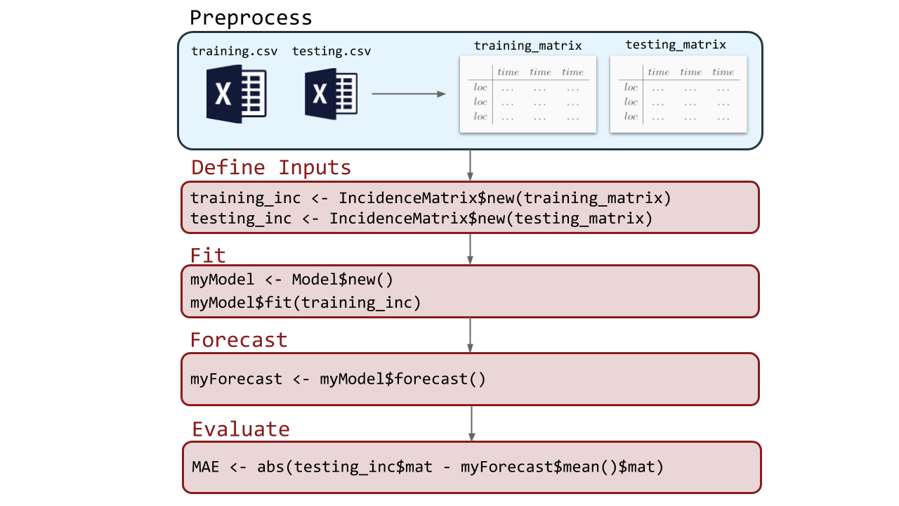

Each of the subsequent vignettes looks into a part of this process. Note that the preprocesing stage will be included in the Defining Inputs Vignette.

Vignette Overview:

The Data
This section will examines the raw data used in the ForecastFramework models ahead.
Defining Inputs: Incidence Matrix
(Beginner Section) This section will define what an Incidence Matrix is, show how to format your data to be used as an Incidence Matrix, and exemplify functions of Incidence Matrices.
Fitting and Forecasting: SARIMATD
(Beginner Section)This section will focus on fitting data to a SARIMA model with ForecastFramework.
Evaluating Complex Models: SARIMATD, SARIMA, GAM
(Intermediate Section) This section will demonstrate evaluation metrics and techniques by comparing two complex models in ForecastFramework.
Creating your own Model: SARIMATD
(Advanced Section) This section will demonstrate how to create your own model with ForecastFramework. NOTE: This section requires object-oriented programming knowledge.

The Data

Demo Data: CDC U.S. Flu Season Data

This demonstration uses influenza surveillance data maintained by the U.S. Centers for Disease Control (CDC). Normally, the data include all 50 US states. For simplicity, this demo only models national data. These data are quickly retrieved with the cdcfluview R package.

One of the measures reported by the CDC for quantifying respiratory illness burden in a population is weighted influenza-like illness (wILI). This is a metric defined as the estimated percentage of all out-patient doctors office visits due to patients who present with “influenza-like illness”, e.g. a fever, a cough and/or sore throat. This wILI percentage, at the national and regional levels, is calculated by taking weighted averages of state-level activty, with weights based on state population.

Raw Data

These data include many attributes, but we will focus on: region,year,week,weighted_ili,week_start. Note that weighted_ili is the wILI measure reported for that specific year and week.

library(cdcfluview)
library(dplyr)
dat <- ilinet(region = "National")
dat <- dat %>%
  select('region','year','week','weighted_ili', 'week_start')
print(head(dat,6))

## # A tibble: 6 x 5
##   region    year  week weighted_ili week_start
##   <chr>    <int> <int>        <dbl> <date>    
## 1 National  1997    40         1.10 1997-09-28
## 2 National  1997    41         1.20 1997-10-05
## 3 National  1997    42         1.38 1997-10-12
## 4 National  1997    43         1.20 1997-10-19
## 5 National  1997    44         1.66 1997-10-26
## 6 National  1997    45         1.41 1997-11-02

Time Series

A time series of the raw data looks like the following:

library(ggplot2)
dat$date_sick <- as.Date(strptime(dat$week_start,"%m/%d/%Y")) # convert to date
plot <- ggplot() +
    geom_line(mapping = aes(x = week_start, y = weighted_ili),
              size=0.7,
              data = dat) +
    xlab("") + ylab("Weighted ILI") +
    coord_cartesian(ylim = c(0, 10)) +
    ggtitle("National Weighted Inluenza-Like Illness")
print(plot)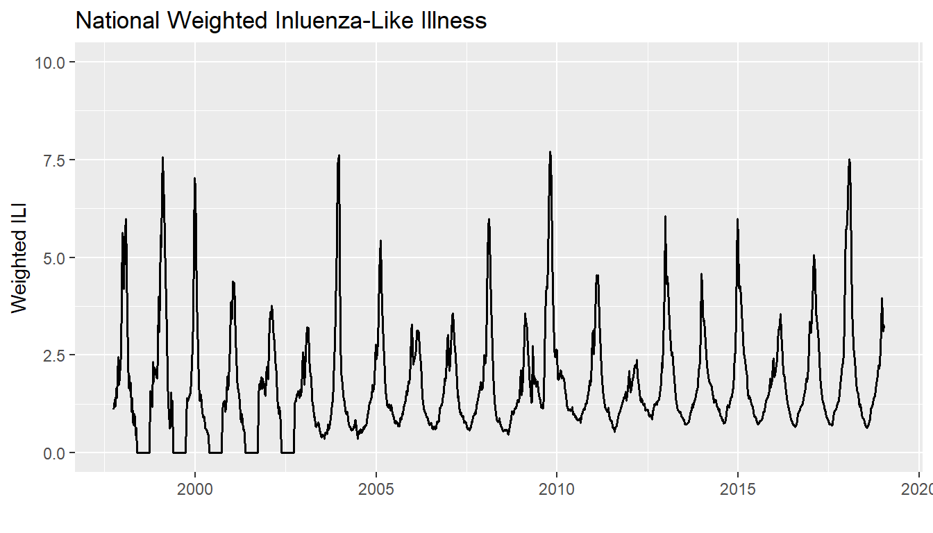

Scope of this demo

This demo will forecast an entire year’s worth of wILI incidence starting from the beginning of the flu season in 2016.

Defining Inputs Incidence Matrix

What is an `IncidenceMatrix`?

ForecastFramework makes it easy to quickly manipulate forecasting data. To do this, create an object from a class called IncidenceMatrix. IncidenceMatrices are the stanard inputs for ForecastFramework models. This vignette describes how to create an IncidenceMatrix and some key fields and methods relating to their usage.

`IncidenceMatrix` in the ForecastFramework Process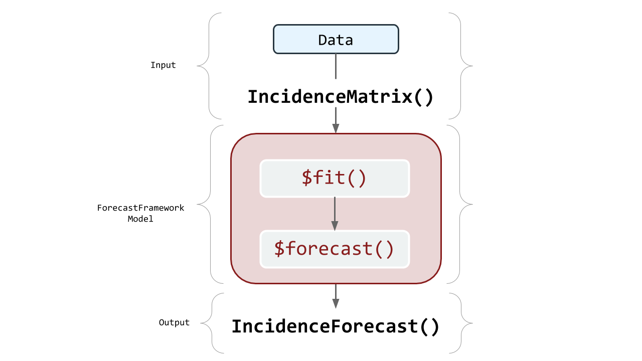

How to create an `IncidenceMatrix`

Make sure you import ForecastFramework and R6

library(R6)

## Warning: package 'R6' was built under R version 3.5.2

library(ForecastFramework)

Create a new matrix with your data

data_matrix <- matrix(1:9,3,3)
print(data_matrix)

##      [,1] [,2] [,3]
## [1,]    1    4    7
## [2,]    2    5    8
## [3,]    3    6    9

Create a new IncidenceMatrix object with your data

data_object <- IncidenceMatrix$new(data_matrix)

List of `IncidenceMatrix` Fields

The IncidenceMatrix class has several fields that can be helpful for data preprocessing.

$mat show data in matrix form
$nrow number of rows
$ncol number of columns
$colData list of metadata associated with the columns of the data
$rowData list of metadata associated with the rows of the data
$cellData list of cell metadata
$cnames names of matrix columns
$rnames names of matrix rows
$metaData any data not part of main matrix

`IncidenceMatrix` Methods

In object oriented programming, a ‘method’ is a function for a class. In this case, the following methods are functions that are applied to IncidenceMatrix.

$addColumns(n) add n columns to matrix
$addRows(n) add n rows to matrix
$diff(n) difference between each column and lag n columns to the left
$lag(n) lag each column by n
$head(k,direction) show x columns/rows from the top (y=1 for columns, 2 for rows)
$tail(k,direction) show x columns/rows from the bottom (y=1 for columns, 2 for rows)
$scale(functin(x){}) scale the matrix by some function
$subset(rows=x,cols=y) take a subset of the matrix by x rows and y columns

Examples of manipulating an `IncidenceMatrix`

Let’s apply some of the example functions from above to our data_object.

$mat show data in matrix form:

data_object$mat

##      [,1] [,2] [,3]
## [1,]    1    4    7
## [2,]    2    5    8
## [3,]    3    6    9

$nrow number of rows in the matrix:

data_object$nrow

## [1] 3

$ncol number of columns in the matrix:

data_object$ncol

## [1] 3

$colData Edit or the column names:

data_object$colData <- list(1:3) # Initialize how many columns headers
data_object$colData <- list(c("A","B","C"))
data_object$colData

## [[1]]
## [1] "A" "B" "C"

$addColumns Edit or the column names:

data_object$addColumns(2)
data_object$colData

## [[1]]
## [1] "A" "B" "C" NA  NA

data_object$mat

##      [,1] [,2] [,3] [,4] [,5]
## [1,]    1    4    7   NA   NA
## [2,]    2    5    8   NA   NA
## [3,]    3    6    9   NA   NA

Fitting and Forecasting

Overview

This demonstration focuses on the simplest building block of any large forecasting experiment or study: how to make a forecast from one model at one time point for a single location. ForecastFramework makes it easy to generalize this process to multiple models, multiple time points and multiple locations. However, for starters, we will focus on the anatomy of a single forecast from a single model.

About sarimaTD

Specifically, we will use a variation on standard Seasonal Auto-Regressive Integrated Moving Average models. sarimaTD is an R package created by Evan Ray. sarimaTD stands for SARIMA with Transformations and Seasonal Differencing. sarimaTD is a model composed of a set of wrapper functions that simplify estimating and predicting traditional SARIMA models. These wrapper functions first transform the incidence data to approximate normality, then perform seasonal differencing (if specified), and input the new incidence data to the auto.arima function from the forecast package. These simple transformations have shown improved forecasting performance of SARIMA models for infectious disease incidence by increasing the numerical stability of the model.

Fitting the ForecastFramework sarimaTD Model

1. Import packages

First you must import all the required libraries. Note that ForecastFramework doesn’t requre dplyr, ggplot2, cdcfluview or RCurl but they will be used for sourcing the models on Github, getting the flu data, and producing the data processing and visualization.

library(ForecastFramework)
library(R6)
library(forecast)
library(dplyr)
library(ggplot2)
library(cdcfluview)

# Source R6 Files
library(RCurl)

# Function of Source Github Models
source_github <- function(u) {
  # read script lines from website and evaluate
  script <- getURL(u, ssl.verifypeer = FALSE)
  eval(parse(text = script),envir=.GlobalEnv)
}  
# Source R6 Files
source_github('https://raw.githubusercontent.com/reichlab/forecast-framework-demos/master/models/ContestModel.R')
source_github('https://raw.githubusercontent.com/reichlab/forecast-framework-demos/master/models/SARIMATD1Model.R')

Now it is time to fit your sarimaTD Model! ForecastFramework makes this easy.

2. Create new sarimaTDmodel Class

In this sarimaTD model, forecasts are created by simulating multiple time-series trajectories from models fit using the forecast::auto.arima() function. Therefore, we must define the number of simulations to generate, nsim. We also need to define the seasonal periodicity of our data, or the period parameter. For this forecast, we know the periodicity is 52, because the data is weekly. once we define these parameters, they can be passed into the sarimaTDModel() class generator to create a new sarimaTDmodel class.

nsim <- 10 # Number of SARIMA simulations 
sarimaTDmodel <- SARIMATD1Model$new(period = 52, nsim = nsim)

3. Import CDC Flu Data

To import the fluview data, use the ilinet() command. The data is then filtered to remove unneeded weeks and years. Then, the data is stored as an IncidenceMatrix. An IncidenceMatrix represents spatial time-series data in a matrix with one row per location and one column per time. To do this, another series of transformations are made. IncidenceMatrix is the preferred input for ForecastFramework Models.

The data will be put into a training, testing, and truth set. The training set will be used to fit the forecast model. The test set is the time period that the model will be forecasting from (this may include the training set). The truth set is the unknown validation data that the used to measure accuracy of the forecast model, this will not include the training data or the testing data. Below is a diagram to differentiate the different test splits: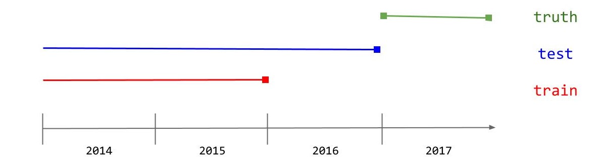

dat <- ilinet(region = "National")
dat <- dat %>% 
  filter( week != 53 &
          year > 2009 & 
          year < 2018 & 
          !(year == 2017 & week > 18))
dat <- dat %>%
  select('region','year','week','weighted_ili', 'week_start')

# Create a Preprocess Function
preprocess_inc <- function(dat){
  dat$time.in.year = dat$week
  dat$t = dat$year + dat$week/52
  inc = ObservationList$new(dat)
  inc$formArray('region','t',val='weighted_ili',
                dimData = list(NULL,list('week','year','time.in.year','t')),
                metaData = list(t.step = 1/52,max.year.time = 52))
  return(inc)
}

# Seperate into Training and Testing Data
training_data <- dat %>% 
  filter( ! ((year == 2016 ) | (year == 2017 ) ))
testing_data <- dat %>% 
  filter( ! ((year == 2016 & week >= 19) | (year == 2017 & week <= 18)) )
truth_data <- dat %>% 
  filter( ((year == 2016 & week >= 19) | (year == 2017 & week <= 18)) )

training_inc <- preprocess_inc(training_data)
testing_inc <- preprocess_inc(testing_data)
truth_inc <- preprocess_inc(truth_data)

Let’s look at a sample from the new IncidenceMatrix to view the IncidenceMatrix Format:

print(training_inc$mat[,0:10])

## 2010.01923076923 2010.03846153846 2010.05769230769 2010.07692307692 
##          1.90712          1.86738          1.88072          1.96908 
## 2010.09615384615 2010.11538461538 2010.13461538462 2010.15384615385 
##          2.11387          2.09695          1.90294          1.96951 
## 2010.17307692308 2010.19230769231 
##          1.92331          1.89659

Notice that the traditional dates have been transformed to fractions of a year.

3. Fit the Model

Typically, different regions would be fit separately and have different forecasts. For the scope of this demo, we are only fitting and forecasting national data.

sarimaTDmodel$fit(training_inc)

Forecasting with the ForecastFramework sarimaTD Model

4. Forecasting SARIMA

Before forecasting, you must specify how many periods ahead you would like to forecast. This is defined by the steps parameter. Then, you forecast with the sarimaTDmodel$forecast() method. This model will forecast one year into the future (26 biweeks).

steps <- 52 # forecast ahead 52 weeks

Then, use the built-in $forecast() function to create your forecasts. This creates a new R6 object with your forecasts and many other useful built-in functions. Be sure to check out the Evaluation section for usage of the Forecasting function.

forecast_X <- sarimaTDmodel$forecast(testing_inc,steps = steps)

Plotting the Output

5. Formatting the Forecast Output

To view the the median forecast of the simulations, execute the following command:

forecast_X$median()$mat

##                1        2        3        4        5        6        7
## National 1.60222 1.517003 1.451777 1.421859 1.282271 1.141956 1.153322
##                 8         9        10        11        12       13
## National 1.147359 0.9795403 0.9668512 0.9520091 0.8279257 0.866433
##                 14        15       16       17       18       19      20
## National 0.8024566 0.8194832 0.825563 0.877521 1.021738 1.132393 1.21812
##                21       22       23       24       25      26       27
## National 1.179522 1.286732 1.342655 1.447219 1.417237 1.43861 1.571644
##                28       29      30       31       32      33       34
## National 1.575276 1.979737 1.97458 2.150017 2.460296 3.12454 3.449338
##                35       36       37       38       39       40       41
## National 2.625559 2.657756 2.747361 2.933748 2.737146 3.014654 3.228957
##                42       43       44      45       46       47       48
## National 2.783363 2.900718 2.962712 2.59425 2.414608 2.307569 2.015418
##                49      50       51       52
## National 1.689113 1.67496 1.602514 1.519792

Lets convert the forecast matrix to a dataframe in R for easy manipulation:

# converting predictions to a dataframe to use dplyr
preds_df <- data.frame(as.table(t(forecast_X$data$mat)))

To include the date_sick in the forecast_X$data$mat output, map the forecast to its predicted dates is to create a new data frame with the data from the missing year. Then, we will combine the output in forecast_X$data with the correct biweek dates.

# converting predictions to a dataframe to use dplyr
# import testing dataset which has 2013 data

# add prediction dates to original forecast
preds_df[["date_sick"]] <-as.Date(truth_data$week_start, format = "%d-%m-%Y")

Now, we can add the forecast to the preds_df. Notice the $median() and $quantile() functions accompanied with $mat will produce matricies with the prediction medians and quantiles, respectively.

preds_df <- preds_df %>%
   mutate( 
      pred_total_cases = as.vector(forecast_X$median(na.rm=TRUE)$mat),
      pred_95_lb = as.vector(forecast_X$quantile(0.025,na.rm=TRUE)$mat),
      pred_95_ub = as.vector(forecast_X$quantile(0.975,na.rm=TRUE)$mat),
      pred_80_lb = as.vector(forecast_X$quantile(0.05,na.rm=TRUE)$mat),
      pred_80_ub = as.vector(forecast_X$quantile(0.95,na.rm=TRUE)$mat),
      pred_50_lb = as.vector(forecast_X$quantile(0.25,na.rm=TRUE)$mat),
      pred_50_ub = as.vector(forecast_X$quantile(0.75,na.rm=TRUE)$mat)
   )
print(head(preds_df,5)) # Print the first 5 rows

##   Var1     Var2     Freq  date_sick pred_total_cases pred_95_lb pred_95_ub
## 1    1 National 1.504730 2016-05-08         1.602220   1.502178   1.771799
## 2    2 National 1.440596 2016-05-15         1.517003   1.367820   1.723899
## 3    3 National 1.309106 2016-05-22         1.451777   1.312411   1.597535
## 4    4 National 1.356588 2016-05-29         1.421859   1.298772   1.557929
## 5    5 National 1.247252 2016-06-05         1.282271   1.166937   1.459569
##   pred_80_lb pred_80_ub pred_50_lb pred_50_ub
## 1   1.502919   1.756320   1.533810   1.714173
## 2   1.370245   1.696371   1.451258   1.529072
## 3   1.315716   1.587900   1.342150   1.541461
## 4   1.302582   1.553202   1.359388   1.441230
## 5   1.183448   1.457517   1.230229   1.392675

6. Plot the Forecast Output

Finally, you are able to plot your sarimaTD Forecast! Lets use ggplot2 to create a cool plot.

Weighted ILI sarimaTD Forecast

data_X_3years <- dat %>% filter(year > 2013)
ggplot(data=preds_df, aes(x=date_sick)) +
  geom_ribbon(
    mapping = aes(ymin = pred_95_lb, ymax = pred_95_ub),
    fill = "cornflowerblue",
    alpha = 0.2) +
  geom_ribbon(
    mapping = aes(ymin = pred_80_lb, ymax = pred_80_ub),
    fill = "cornflowerblue",
    alpha = 0.2) +
  geom_ribbon(
    mapping = aes(ymin = pred_50_lb, ymax = pred_50_ub),
    alpha = 0.2) +
  geom_line(
    mapping = aes(y = pred_total_cases),
    color = "royalblue",
    size = 2) +
  geom_line(aes(x = week_start, y = weighted_ili),
            size=0.7,
            data = data_X_3years) +
  xlab("") + ylab("Weighted ILI")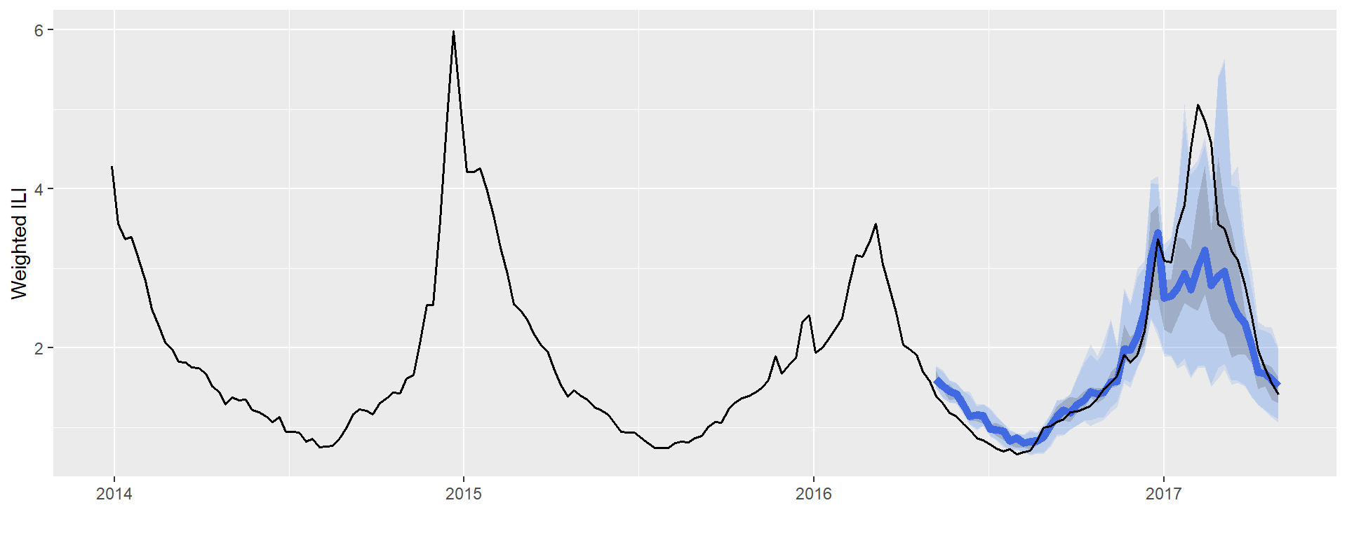

Evaluating Multiple Models

This tutorial will demonstrate how to easily compare multiple models on ForecastFramework. One of the best advantages of ForecastFramework is the ability to evaluate many models at once with the same functions.

Preprocessing Data

Import libraries and source models

library(ForecastFramework)
library(R6)
library(forecast)
library(dplyr)
library(ggplot2)
library(cdcfluview)
library(gridExtra)
library(data.table)
library(knitr)
library(kableExtra)
library(RCurl)

# Function of Source Github Models
source_github <- function(u) {
  # read script lines from website and evaluate
  script <- getURL(u, ssl.verifypeer = FALSE)
  eval(parse(text = script),envir=.GlobalEnv)
}  
# Source R6 Files
source_github('https://raw.githubusercontent.com/reichlab/forecast-framework-demos/master/models/ContestModel.R')
source_github('https://raw.githubusercontent.com/reichlab/forecast-framework-demos/master/models/AggregateForecastModel.R')
source_github('https://raw.githubusercontent.com/reichlab/forecast-framework-demos/master/models/SARIMAModel.R')
source_github('https://raw.githubusercontent.com/reichlab/forecast-framework-demos/master/models/GamModel.R')
source_github('https://raw.githubusercontent.com/reichlab/forecast-framework-demos/master/models/SARIMATD1Model.R')

Upload data from cdcfluview as dataframes. In this demo, we are only concerned with years between 2010 and 2017. We split training, testing, and truth data by excluding the 2016-17 Flu season in the truth set.

# Seperate into Training and Testing Data
dat <- ilinet(region = "National")
dat <- dat %>% 
  filter( week != 53 &
          year > 2009 & 
          year < 2018 & 
          !(year == 2017 & week > 18))
dat <- dat %>%
  select('region','year','week','weighted_ili', 'week_start')

# Seperate into Training, Testing, and Truth Data
training_data <- dat %>% 
  filter( ! ((year == 2016 ) | (year == 2017 ) ))
testing_data <- dat %>% 
  filter( ! ((year == 2016 & week >= 19) | (year == 2017 & week <= 18)) )
truth_data <- dat %>% 
  filter( ((year == 2016 & week >= 19) | (year == 2017 & week <= 18)) )

A sample of the data we are forecasting.

head(testing_data,5)

## # A tibble: 5 x 5
##   region    year  week weighted_ili week_start
##   <chr>    <int> <int>        <dbl> <date>    
## 1 National  2010     1         1.91 2010-01-03
## 2 National  2010     2         1.87 2010-01-10
## 3 National  2010     3         1.88 2010-01-17
## 4 National  2010     4         1.97 2010-01-24
## 5 National  2010     5         2.11 2010-01-31

Then, preprocess the training, testing, and truth dataframes to become new incidence matrices. This script uses the ObservationList$new() ForecastFramework function to easily convert the dataframe to an IncidenceMatrix. The $formArray() is the second step to complete the IncidenceMatrix.

Note: The time step in this example is 52 weeks; however, there are datasets with other timesteps (e.g. 26 biweeks) that would impact the calculations of t.step, dat$t, and max.year.time values.

# Create a Preprocess Function
preprocess_inc <- function(dat){
  dat$time.in.year = dat$week
  dat$t = dat$year + dat$week/52
  inc = ObservationList$new(dat)
  inc$formArray('region','t',val='weighted_ili',
                dimData = list(NULL,list('week','year','time.in.year','t')),
                metaData = list(t.step = 1/52,max.year.time = 52))
  return(inc)
}

training_inc <- preprocess_inc(training_data)
testing_inc <- preprocess_inc(testing_data)
truth_inc <- preprocess_inc(truth_data)

Defining Models

This demo will be evaluating the Generalized Additive Model (GAM), SARIMA, and sarimaTD models given different evaluation metrics. The GAM model is based on the model used in published real-time infectious disease forecasting research.

# Defining the Models
nsim <- 1000 # Number of simulations 
region_num <- 1 # Only modeling the "National" region
time_step <- 52

sarimaTD_model <- SARIMATD1Model$new(period = time_step, nsim = nsim)
sarima_model <- SARIMAModel$new(period = time_step, nsim = nsim)
gam_model <- GamModel$new(numProvinces = region_num, nSims = nsim)

Fitting Models

Each model is fit with the training data.

# Fit the Models 
sarimaTD_model$fit(training_inc) # Fitting this model will take awhile
sarima_model$fit(training_inc)
gam_model$fit(training_inc)

Forecasting Models

We are forecasting from the beginning of flu season 2016-17, 52 weeks into the future.

# Forecasting the Models
steps <- 52 # forecast ahead 26 biweeks
forecast_sarimaTD <- sarimaTD_model$forecast(testing_inc, step = steps)
forecast_sarima <- sarima_model$forecast(testing_inc, step = steps)
forecast_gam <- gam_model$forecast(testing_inc, step = steps)

Evaluating the Models

Now for the fun part! How did the models perform? This question is easy to answer with ForecastFramework Models.

Important Note: This is not a formal model evaluation or comparison. The goal of this exercise is to demonstrate different ForecastFramework techniques. Although the sarimaTD model appears to perform better than the other models in this example, a more in-depth analysis must be made before any conclusions can be made about model performance.

Side-by-Side Forecasting Timeseries This function creates a time series visualization with the predicted median and quantiles displayed by a specific color. Notice forecast$quantile(0.025)$mat gives a matrix with a 2.5% quantile. Additionally, forecast$mean()$mat gives the mean forecast for that specific time period. Additionally, na.rm=TRUE, removes any NA values in the simulation to calculate the mean.

# Function to create time series with Visualization
visualize_model <- function(forecast, rib_color, main_color){
  data_X_3years <- dat %>% filter(year > 2013)
  preds_df <- data.frame(as.table(t(forecast$data$mat)))
  preds_df[["week_start"]] <-as.Date(truth_data$week_start, format = "%Y-%d-%m")
  preds_df <- preds_df %>%
    mutate( 
      pred_total_cases = as.vector(forecast$mean(na.rm=TRUE)$mat),
      pred_95_lb = as.vector(forecast$quantile(0.025,na.rm=TRUE)$mat),
      pred_95_ub = as.vector(forecast$quantile(0.975,na.rm=TRUE)$mat),
      pred_80_lb = as.vector(forecast$quantile(0.05,na.rm=TRUE)$mat),
      pred_80_ub = as.vector(forecast$quantile(0.95,na.rm=TRUE)$mat),
      pred_50_lb = as.vector(forecast$quantile(0.25,na.rm=TRUE)$mat),
      pred_50_ub = as.vector(forecast$quantile(0.75,na.rm=TRUE)$mat)
    )
  plot <- ggplot() +
    geom_ribbon(
      mapping = aes(x = week_start, ymin = pred_95_lb, ymax = pred_95_ub),
      fill = rib_color,
      alpha = 0.2,
      data = preds_df) +
    geom_ribbon(
      mapping = aes(x = week_start, ymin = pred_80_lb, ymax = pred_80_ub),
      fill = rib_color,
      alpha = 0.2,
      data = preds_df) +
    geom_ribbon(
      mapping = aes(x = week_start, ymin = pred_50_lb, ymax = pred_50_ub),
      fill = rib_color,
      alpha = 0.2,
      data = preds_df) +
    geom_line(
      mapping = aes(x = week_start, y = pred_total_cases),
      color = main_color,
      size = 1,
      data = preds_df) + 
    geom_line(mapping = aes(x = week_start, y = weighted_ili),
              size=0.7,
              data = data_X_3years) +
    xlab("") + ylab("Weighted ILI") + coord_cartesian(ylim = c(0, 13))
  return(plot)
}

# Create each plot
plot1 <- visualize_model(forecast_sarimaTD, "palegreen3", "forestgreen") + ggtitle("sarimaTD")
plot2 <- visualize_model(forecast_sarima, "coral1", "red") + ggtitle("SARIMA")
plot3 <- visualize_model(forecast_gam, "cornflowerblue" , "blue")+ ggtitle("GAM")

# Display side-by-side plots
grid.arrange(plot1, plot2, plot3, ncol=3)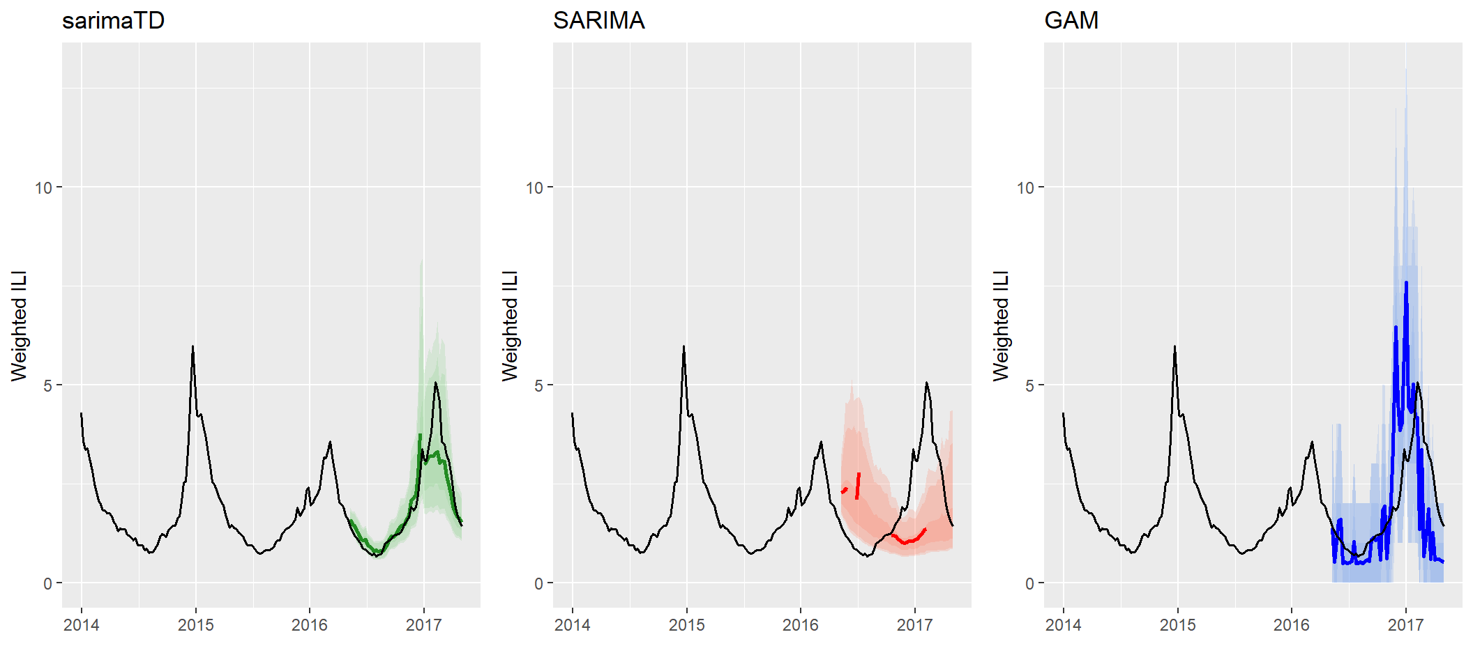

Note the sparsity in the SARIMA forecast, due to some forecasted trajectories yielding undefined forecasted means (e.g. if one of the trajectories contains a non-numeric or NA value). This is one benefit of sarimaTD - the ability to provide stable long-term forecasts with the aid of transformations and seasonal differencing. It avoids some of the “brittlenes” that we have observed when just using SARIMA fitting out of the box.

Common Evaluation Metrics Calculating evaluation metrics is easy with ForecastFramework objects.

# Mean Absolute Error
MAE <- function(forecast_mean, test_inc){
  err <- test_inc$mat-forecast_mean
  abs_err <- abs(err)
  return(mean(abs_err))
}
# Mean Squared Error
MSE <- function(forecast_mean, test_inc){
  err <- test_inc$mat-forecast_mean
  err_sq <- err^2
  return(mean(err_sq))
}
# Mean Absolute Percentage Error
MAPE <- function(forecast_mean, test_inc){
  err <- test_inc$mat-forecast_mean
  abs_err <- abs(err)
  abs_err_percent <- abs_err/test_inc$mat
  return(mean(abs_err_percent)*100)
}
# Root Mean Squared Error
RMSE <- function(forecast_mean, test_inc){
  err <- test_inc$mat-forecast_mean
  err_sq <- err^2
  mse <-mean(err_sq)
  return(sqrt(mse))
}

Each Model can be evaluated given the various functions:

# Create Arrays with each Metric
evaluate <- function(forecast){
  # Replace any NaN values with 0
  forecast_mat <- forecast$mean(na.rm=TRUE)$mat
  forecast_mat[is.na(forecast_mat)] <- 0
  
  # Evaluate Performance
  MAE <- MAE(forecast_mat, truth_inc)
  MSE <- MSE(forecast_mat, truth_inc)
  MAPE <- MAPE(forecast_mat, truth_inc)
  RMSE <- RMSE(forecast_mat, truth_inc)
  return(c(MAE,MSE,MAPE,RMSE))
}

gam_eval <- evaluate(forecast_gam)
sarimaTD_eval <- evaluate(forecast_sarimaTD)
sarima_eval <- evaluate(forecast_sarima)

Then, a final Table is made with all of the metrics in a grid format:

	sarimaTD	SARIMA	GAM
MAE	0.3799110	1.586660	1.044438
MSE	0.4865753	3.760848	2.249297
MAPE	15.9814438	85.486579	50.098176
RMSE	0.6975495	1.939291	1.499766

Creating your own Model

Creating your Own Model

This Tutorial will demonstrate how to create a basic model with ForecastFramework. Models are created with R Object-Oriented programming, or the R6 package. It is essential to have a basic understanding of the structure of R6 Objects, before creating a ForecastFramework package. In this tutorial, the SARIMATD model will be created step-by-step.

SARIMATD

SARIMATD is a model created by Evan Ray. SARIMATD uses set of wrapper functions around the forecast package to simplify estimation of and prediction from SARIMA models.

Basic Steps of the Model:

Incidence data are transformed to approximate normality
Seasonal differencing is performed
Transformed data are passed to forecast::auto.arima for model selection and estimation simulate trajectories of future incidence

Building the SARIMATD Model

1. Start with an Empty Model

ForecastFramework models all have the same basic structure:

model <- R6Class(
  inherit = ContestModel, # or AggregateModel
  private = list(
    #' private section is for aspects we do not want the user to access directly
  ),
  public = list(
    #' @method fit_ Get the model ready to forecast
    #' @param data The data to fit the model to.
    fit = function(data){
      ...
    },
    #' @method forecast Predict some number of time steps into the future.
    #' @param newdata The data to forecast from
    #' @param steps The number of timesteps into the future to forecast
    forecast = function(newdata,steps){
      ...
    },
    #' @method initialize Create a new instance of this class. 
    initialize = function(){
      ...
    }
  )
)

2. Define your `fit()` and `forecast()` functions

The easiest way to incorporate a model into ForecastFramework is to pre-define your fit and forecast functions in a separate package, or use a separate package like the forecast package. The SARMATD package is hosted on GitHub and available for download with CRAN.

The SARIMATD fit function is as follows:

#' @param y a univariate time series or numeric vector.
#' @param ts_frequency frequency of time series.  Must be provided if y is not
#'   of class "ts".  See the help for stats::ts for more.
#' @param transformation character specifying transformation type:
#'   "box-cox", "log", "forecast-box-cox", or "none".  See details for more.
#' @param seasonal_difference boolean; take a seasonal difference before passing
#'   to auto.arima?
#' @param auto.arima_d order of first differencing argument to auto.arima.
#' @param auto.arima_D order of seasonal differencing argument to auto.arima.
fit_sarima(
          y,
          ts_frequency,
          transformation = "box-cox",
          seasonal_difference = TRUE,
          d = NA,
          D = NA)

The SARIMATD forecast function is as follows (note that SARIMATD is a simulated forecast):

#' @param object a sarima fit of class "sarima_td", as returned by fit_sarima
#' @param nsim number of sample trajectories to simulate
#' @param seed either `NULL` or an integer that will be used in a call to
#'   `set.seed` before simulating the response vectors.  If set, the value is
#'   saved as the "seed" attribute of the returned value.  The default, `Null`,
#'   will not change the random generator state, and return `.Random.seed`
#'   as the "seed" attribute
#' @param newdata new data to simulate forward from
#' @param h number of time steps forwards to simulate
#'
#' @return an nsim by h matrix with simulated values
simulate.sarimaTD(
                  object,
                  nsim = 1,
                  seed = NULL,
                  newdata,
                  h = 1)

3. Update the R6 Private Section

This section of the Model:

 private = list(
    #' @method private section is for aspects we do not want the user to access directly
  ),

Will become:

  private = list(
    .data = NULL,        ## every model should have this
    .models = list(),    ## specific to models that are fit separately for each location
    .nsim = 1000,        ## models that are simulating forecasts need this
    .lambda = list(),    ## specific to ARIMA models
    .period = integer(0) ## specific to SARIMA models
  ),

This section is comprised of inputs in your model that are not able to be accessed by the user directly, but will be updatable in the later initialize section. The arguments in the fit() and forecast() functions are fixed without incorporating private fields. For example, the nsim (number of simulations) may change, which makes it necessary to add these updatable variables in the private section. However, notice that all private variables include a . in the private section. This is the common way of distinguising a private variable in R6.

4. Update the fit Method

Upload IncidenceMatrix to Fit function:

 fit = function(data) {
      ## All fit functions should have this, it helps with debugging
      if("fit" %in% private$.debug){browser()}
      
      ## stores data for easy access and checks to make sure it's the right class
      private$.data <- IncidenceMatrix$new(data)
      
 }

Cycle though each province and use the fit_sarima() function.

 fit = function(data) {
      ## All fit functions should have this, it helps with debugging
      if("fit" %in% private$.debug){browser()}
    
      ## stores data for easy access and checks to make sure it's the right class
      private$.data <- IncidenceMatrix$new(data)
      
      ## for each location/row
      for (row_idx in 1:private$.data$nrow) {
        ### need to create a y vector with incidence at time t
        y <- private$.data$subset(rows = row_idx, mutate = FALSE)
        
        ## private$.models[[row_idx]] <- something
        y_ts <- ts(as.vector(y$mat), frequency = private$.period)
        private$.lambda[[row_idx]] <- BoxCox.lambda(y_ts)
        private$.models[[row_idx]] <- fit_sarima(y = y_ts,
                                                 transformation = "box-cox",
                                                 seasonal_difference = TRUE)
      }
 }

4. Update the forecast Method

Using the pre-defined equation simulate.sarimaTD() for the forecast method. nmodels, sim_forecasts and dimnames(simforecasts) are all variables needed to define a simulated forecast in ForecastFramework.

    forecast = function(newdata = private$.data, steps) {
      ## include for debugging
      if("forecast" %in% private$.debug){browser()} 
      
      ## number of models (provinces) to forecast
      nmodels <- length(private$.models)
      
      ## define an array to store the simulated forecasts
      sim_forecasts <- array(dim = c(nmodels, steps, private$.nsim))
      dimnames(sim_forecasts) <- list(newdata$rnames, 1:steps, NULL)
      
    }

Now, the Provinces are iterated through and simulated with the simulate.sarimaTD()function (called as just simulate()). Then, there are a couple of matrix transformations to input the simulated matrix into the SimulatedIncidenceMatrix() Object.

    forecast = function(newdata = private$.data, steps) {
      ## include for debugging
      if("forecast" %in% private$.debug){browser()} 
      
      ## number of models (provinces) to forecast
      nmodels <- length(private$.models)
      
      ## define an array to store the simulated forecasts
      sim_forecasts <- array(dim = c(nmodels, steps, private$.nsim))
      dimnames(sim_forecasts) <- list(newdata$rnames, 1:steps, NULL)
      
      ## iterate through each province and forecast with simulate.satimaTD
      for(model_idx in 1:length(private$.models)) {
          tmp_arima <-  simulate(object = private$.models[[model_idx]],
                                 nsim = private$.nsim,
                                 seed = 1,
                                 newdata = as.vector(newdata$mat[model_idx,]),
                                 h = steps
                                )
          ## transpose simulate() output to be consistent with ForecastFramework
          tmp_arima <- t(tmp_arima)
          sim_forecasts[model_idx, , ] <- tmp_arima
      }
      private$output <- SimulatedIncidenceMatrix$new(sim_forecasts)
      return(IncidenceForecast$new(private$output, forecastTimes = rep(TRUE, steps)))
    }

5. Update the initialize Method

The initialize method is to initialize inputs. In this case, one input that needs initialization is the period (number of biweeks).

initialize = function(period = 26, nsim=1000) { 
      ## this code is run during SARIMAModel$new()
      ## need to store these arguments within the model object
      private$.nsim <- nsim
      private$.period <- period
    },

6. Update the active binding

We will ignore this section for now. It is a more advanced level and stay tuned for another vignette that expains active binding.

7. Putting everything Together

All of the previous sections and methods are put together as the R6 Object:

library(ForecastFramework)
library(R6)
library(forecast)
library(sarimaTD)

# SARIMATDModel Description:
# Implementation of the sarimaTD model created by Evan Ray
# More information about sarimaTD in https://github.com/reichlab/sarimaTD 
# Integrated into ForecastFramework by: Katie House, 6/22/2018

SARIMATD1Model <- R6Class(
  inherit = ContestModel,
  private = list(
    .data = NULL,        ## every model should have this
    .models = list(),    ## specific to models that are fit separately for each location
    .nsim = 1000,        ## models that are simulating forecasts need this
    .period = integer(0) ## specific to SARIMA models
  ),
  public = list(
    ## data will be MatrixData
    fit = function(data) {
      if("fit" %in% private$.debug){browser()}
      ## stores data for easy access and checks to make sure it's the right class
      private$.data <- IncidenceMatrix$new(data)
      
      ## for each location/row
      for (row_idx in 1:private$.data$nrow) {
        ### need to create a y vector with incidence at time t
        y <- private$.data$subset(rows = row_idx, mutate = FALSE)
        
        ## convert y vector to time series data type
        y_ts <- ts(as.vector(y$mat), frequency = private$.period)
        
        ## fit sarimaTD with 'fit_sarima()' from sarimaTD package
        ## fit_sarima() performs box-cox transformation and seasonal differencing
        private$.models[[row_idx]] <- fit_sarima(y = y_ts,
                                                 transformation = "box-cox",
                                                 seasonal_difference = TRUE)
      }
    },
    forecast = function(newdata = private$.data, steps) {
      ## include for debugging
      if("forecast" %in% private$.debug){browser()} 
      
      ## number of models (provinces) to forecast
      nmodels <- length(private$.models)
      
      ## define an array to store the simulated forecasts
      sim_forecasts <- array(dim = c(nmodels, steps, private$.nsim))
      dimnames(sim_forecasts) <- list(newdata$rnames, 1:steps, NULL)
      
      ## iterate through each province and forecast with simulate.satimaTD
      for(model_idx in 1:length(private$.models)) {
          tmp_arima <-  simulate(object = private$.models[[model_idx]],
                                 nsim = private$.nsim,
                                 seed = 1,
                                 newdata = as.vector(newdata$mat[model_idx,]),
                                 h = steps
                                )
          ## transpose simulate() output to be consistent with ForecastFramework
          tmp_arima <- t(tmp_arima)
          sim_forecasts[model_idx, , ] <- tmp_arima
      }
      private$output <- SimulatedIncidenceMatrix$new(sim_forecasts)
      return(IncidenceForecast$new(private$output, forecastTimes = rep(TRUE, steps)))
    },
    initialize = function(period = 26, nsim=1000) { 
      ## this code is run during SARIMAModel$new()
      ## need to store these arguments within the model object
      private$.nsim <- nsim
      private$.period <- period
    }
  )
)

8. Testing the New Model

Lets now test the model on the same biweek counts as the SARIMA demo. The output is a forecasted case count for 26 biweeks.

# training data for province 10, years 2006 - 2012 
library(ForecastFramework)
library(R6)
library(forecast)
library(dplyr)
library(ggplot2)
library(cdcfluview)

# Source R6 Files
library(RCurl)

# Function of Source Github Models
source_github <- function(u) {
  script <- getURL(u, ssl.verifypeer = FALSE)
  eval(parse(text = script),envir=.GlobalEnv)
}  
# Source R6 Files
source_github('https://raw.githubusercontent.com/reichlab/forecast-framework-demos/master/models/ContestModel.R')
source_github('https://raw.githubusercontent.com/reichlab/forecast-framework-demos/master/models/SARIMATD1Model.R')

# Preprocess data to Inc Matrix
data2 <- ilinet(region = "National")
data2 <- data2 %>% filter( week != 53)
data2 <- data2 %>% 
  filter( year > 2009 & 
          year < 2018 & 
          !(year == 2017 & week > 18))
data2 <- data2 %>%
  select('region','year','week','weighted_ili', 'week_start')

preprocess_inc <- function(dat){
  dat$time.in.year = dat$week
  dat$t = dat$year + dat$week/52
  inc = ObservationList$new(dat)
  inc$formArray('region','t',val='weighted_ili',
                dimData = list(NULL,list('week','year','time.in.year','t')),
                metaData = list(t.step = 1/52,max.year.time = 52))
  return(inc)
}
training_data <- data2 %>% 
  filter( ! ((year == 2016 & week >= 19)| (year == 2017 ) ))
training_inc <- preprocess_inc(training_data)

# Create new SARIMATD model
nsim <- 10 # Number of SARIMA simulations 
sarimaTD_model <- SARIMATD1Model$new(period = 52, nsim = nsim)

# Fit SARIMATD model
sarimaTD_model$fit(training_inc)

# Forecast SARIMATD Model
steps <- 52 # forecast ahead 26 biweeks
forecast_X <- sarimaTD_model$forecast(steps = steps)

print(forecast_X$data$mat)

##                 1        2        3        4       5        6        7
## National 1.506281 1.435443 1.304374 1.347654 1.24714 1.070886 1.096122
##                 8        9        10       11        12        13
## National 1.157917 1.047976 0.9764447 1.040178 0.9635555 0.9419319
##                 14        15        16        17       18       19
## National 0.8034576 0.8898613 0.8507697 0.8987568 1.039316 1.235505
##                20       21       22       23       24       25       26
## National 1.361213 1.424291 1.601538 1.758629 1.579438 1.744609 1.689507
##                27       28       29       30       31       32       33
## National 1.737789 1.599809 1.834851 1.946455 2.163725 2.501603 3.381165
##               34       35       36      37      38       39       40
## National 3.83878 2.527224 2.610964 2.57757 2.59635 2.874639 3.215275
##                41       42       43       44       45       46       47
## National 3.184312 2.996799 3.373688 3.607115 2.898903 2.553172 2.446302
##                48       49       50       51       52
## National 2.176144 1.937228 1.939763 1.910833 1.678264

<a title="shopify site analytics"
   href="http://statcounter.com/shopify/" target="_blank">
  <img class="statcounter"
       src="http://c.statcounter.com/10491184/0/40c0ea38/1/"
       alt="shopify site analytics">
</a>

ForecastFramework Demo

About ForecastFramework

Purpose

Usage

Creation

Getting Started

Installation of Forecast Framework

Run this to ensure you have all the Dependencies

The ForecastFramework Pipeline

Vignette Overview:

The Data

Defining Inputs: Incidence Matrix

Fitting and Forecasting: SARIMATD

Evaluating Complex Models: SARIMATD, SARIMA, GAM

Creating your own Model: SARIMATD

The Data

Demo Data: CDC U.S. Flu Season Data

Raw Data

Time Series

Scope of this demo

Defining Inputs Incidence Matrix

What is an IncidenceMatrix?

IncidenceMatrix in the ForecastFramework Process

How to create an IncidenceMatrix

List of IncidenceMatrix Fields

IncidenceMatrix Methods

Examples of manipulating an IncidenceMatrix

Fitting and Forecasting

Overview

About sarimaTD

Fitting the ForecastFramework sarimaTD Model

1. Import packages

2. Create new sarimaTDmodel Class

3. Import CDC Flu Data

3. Fit the Model

Forecasting with the ForecastFramework sarimaTD Model

4. Forecasting SARIMA

Plotting the Output

5. Formatting the Forecast Output

6. Plot the Forecast Output

Weighted ILI sarimaTD Forecast

Evaluating Multiple Models

Evaluating Multiple Models

Preprocessing Data

Defining Models

Fitting Models

Forecasting Models

Evaluating the Models

Creating your own Model

Creating your Own Model

SARIMATD

Building the SARIMATD Model

1. Start with an Empty Model

2. Define your fit() and forecast() functions

3. Update the R6 Private Section

4. Update the fit Method

4. Update the forecast Method

5. Update the initialize Method

6. Update the active binding

7. Putting everything Together

8. Testing the New Model

What is an `IncidenceMatrix`?

`IncidenceMatrix` in the ForecastFramework Process

How to create an `IncidenceMatrix`

List of `IncidenceMatrix` Fields

`IncidenceMatrix` Methods

Examples of manipulating an `IncidenceMatrix`

2. Define your `fit()` and `forecast()` functions